Starting With Data
Last updated on 2024-06-18 | Edit this page
Overview
Questions
- How can I import data in Python?
- What is Pandas?
- Why should I use Pandas to work with data?
Objectives
- Navigate the workshop directory and download a dataset.
- Explain what a library is and what libraries are used for.
- Describe what the Python Data Analysis Library (Pandas) is.
- Load the Python Data Analysis Library (Pandas).
- Use
read_csvto read tabular data into Python. - Describe what a DataFrame is in Python.
- Access and summarize data stored in a DataFrame.
- Define indexing as it relates to data structures.
- Perform basic mathematical operations and summary statistics on data in a Pandas DataFrame.
- Create simple plots.
Working With Pandas DataFrames in Python
We can automate the processes listed above using Python. It is efficient to spend time building code to perform these tasks because once it is built, we can use our code over and over on different datasets that share a similar format. This makes our methods easily reproducible. We can also share our code with colleagues so they can replicate our analysis.
Starting in the same spot
If you do not already have JupyterLab opened from the workshop directroy, let’s do that now. Doing so should help us avoid path and file name issues. At this time please navigate to the workshop directory in your terminal.
Opening JupyterLab
BASH
# navigate to or start your terminal from the worskhop directory
$ jupyter lab
# you may see various status messages as it spins up jupyter server
# and launches your default browser
A quick aside that there are Python libraries like OS Library that can work with our directory structure, however, that is not our focus today.
Alex: our user story
Alex is a researcher interested in exploring the collection of fictional works at their university and assessing how representative it is in relation to the student body. Alex was able to find a pre-liminary dataset assembled by a previous researcher from which they want to create some exploratory plots and intermediate datasets in order to determine next steps to expand on this line of inquiry.
Alex could do some of this work using spreadsheet systems but this can be time consuming to do and lead to mistakes that are hard to detect.
This workshop will show how Python can be used to automate some of the processes allowing them to be re-run in the future.
Our Data
We will be using files from the data folder. This section will use
the all_works.csv file that can be found in your data
folder.
The dataset is stored as a comma separated (.csv) file,
where each row holds information for a single title, and the columns
represent diferent aspects (variables) of each entry:
| Column | Description |
|---|---|
| title | Title of Work |
| subjects | List of Subjects |
| mms_id | Metadata Management System ID |
| author | Author(s) delimited with ‘;’ |
| publication_date | Year of Publication |
| publication_place | Place of Publication |
| language_code | Language of Text |
| resource_type | Type of resource, e.g. physical, electronic |
| acquisition_date | Date of Acquisition |
| is_dei | Boolean for whether work meets broadest definition of a DEI work |
| checkouts | Count of number of times |
Semantics of DEI
- Diversity, Equity and Inclusion are not concrete terms that can be
divorced from history and geography. Thus, it is incumbent on academic
researchers to define what that means in their practice.
- Arguably, any resource is potentially useful in the pursuit of DEI
research if for no other reason as to provide contrast and foreground
for other works, so designating something a DEI resource will always be
a judgment call.
- Here, though, the is_dei flag is applied to any works with subjects deemed outside those with a male, western European lineage. That determination is also a judgment call on multiple levels that you may disagree with, and that is okay. Not only might you disagree with what subjects do or do not share a male, western European lineage, but we are also at the mercy of the cataloger wrestling with their own biases while applying a limited scope of slowly evolving options.
- Our flag will never be perfect, so our goal should be good enough with the time and information we have. You can spot check the subjects deemed dei and non-dei.
- All datasets should be approached with a sceptical eye. When we are done here, you should not only know how to leverage datasets, but interogate and adjust them to adhere to different assumptions. Just be sure to make those adjustments and assumptions clear to those who follow after you.
If we open the all_works.csv data file using a text
editor, the first few rows of our first file look like this:
title,subjects,mms_id,author,publication_date,publication_place,language_code,resource_type,acquisition_date,is_dei,subject_count,chekcouts
"""A god of justice?"" : the problem of evil in twentieth-century Black literature","['American literature--African American authors--History and criticism', 'African Americans--Intellectual life--20th century', 'African Americans--Intellectual lif', 'American literature--African American author']",991004617919702908,"Whitted, Qiana J., 1974-",2009.0,Charlottesville,eng,Book - Physical,2016-06-26 23:51:01,True,4,
"""Baad bitches"" and sassy supermamas : Black power action films","['Blaxploitation films--United States--History and criticism', 'African American women heroes in motion pictures', 'African American women heroes in motion picture', 'Blaxploitation film', 'Blaxploitation Film']",991003607949702908,"Dunn, Stephane, 1967-",2008.0,Urbana,eng,Book - Physical,2011-12-13 03:51:20,True,5,1.0
"""Codependent lesbian space alien seeks same""","['Lesbians--Drama', 'Lesbians', 'Video recordings for the hearing impaired']",991013190057102908,"Olnek, Madeleine.; Space Aliens, LLC.",2011.0,"[New York, NY?]",eng,Projected medium - Physical,2016-11-10 07:56:09,True,3,1.0
"""Lactilla tends her fav'rite cow"" : ecocritical readings of animals and women in eighteenth-century British labouring-class women's poetry","['English poetry--Women authors--History and criticism', 'Working class writings, English--History and criticism', 'Ecofeminism in literature', 'English poetry--Women authors', 'Working class women in literature', 'Working class writings, English']",991003662979702908,"Milne, Anne.",2008.0,Lewisburg,eng,Book - Physical,2015-10-07 16:31:28,True,8,
Why software libraries
Theoretically, you could use only built in python functions to interact directly with the text file, but you would be re-inventing the wheel. Better to do a little research and find someone who has already grappled with similar problems and stand on their shoulders instead. Programming often has a mechanism to facilitate this. In python, the are called libraries.
A library in Python contains a set of tools (functions) that perform different actions. Importing a library is like getting a set of particular tools out of a storage locker and setting them up on the bench for use in a project. Once a library is set up, its functions can be used or called to perform different tasks.
Why Pandas in Python
One of the best options for working with tabular data in Python is to use the Python Data Analysis Library (a.k.a. Pandas Library). The Pandas library provides structures to sort our data, can produce high quality plots in conjunction with other libraries such as matplotlib, and integrates nicely with libraries that use NumPy (which is another common Python library) arrays.
Loading a library
Python doesn’t load all of the libraries available to it by default.
We have to add an import statement to our code in order to
use library functions required for our project. To import a library, we
use the syntax import libraryName, where
libraryName represents the name of the specific library we
want to use. Note that the import command calls a library
that has been installed previously in our system. If we use the
import command to call for a library that does not exist in
our local system, the command will throw and error when executed. In
this case, you can use pip command in another terminal
window to install the missing libraries. See
here for details on how to do this.
Moreover, if we want to give the library a nickname to shorten the
command, we can add as nickNameHere. An example of
importing the pandas library using the common nickname pd
is:
Each time we call a function that’s in a library, we use the syntax
LibraryName.FunctionName. Adding the library name with a
. before the function name tells Python where to find the
function. In the example above, we have imported Pandas as
pd. This means we don’t have to type out
pandas each time we call a Pandas function.
Reading CSV Data Using Pandas
We will begin by locating and reading in a data which in CSV format.
We can use Pandas’ read_csv function to pull either a local
(a file in our machine) or a remote (one that is available for
downloading from the web) file into a Pandas table or DataFrame.
In order to read data in, we need to know where the data is stored on our computer or its URL address if the file is available on the web.
PYTHON
# note that pd.read_csv is used because we imported pandas as pd
# note that this assumes that the data file is in the same location
# as the Jupyter notebook to simplify pathing
pd.read_csv("all_works.csv")
So What’s a DataFrame?
A DataFrame is a 2-dimensional data structure that can store data of
different types (including characters, integers, floating point values,
factors and more) in columns. It is similar to a spreadsheet or a
data.frame in R. A DataFrame always has an index (0-based
integers by default). An index refers to the position of an element in
the data structure.
The above command yields the output similar to below, but formatted differently
                                                   title                                           subjects  ...  is_dei checkouts
0      "A god of justice?" : the problem of evil in t...  ['American literature--African American author...  ...    True         0
1      "Baad bitches" and sassy supermamas : Black po...  ['Blaxploitation films--United States--History...  ...    True         1
2           "Codependent lesbian space alien seeks same"  ['Lesbians--Drama', 'Lesbians', 'Video recordi...  ...    True         1
3      "Lactilla tends her fav'rite cow" : ecocritica...  ['English poetry--Women authors--History and c...  ...    True         0
4      "The useless mouths", and other literary writings  ['French drama--20th century--Translations int...  ...    True         1
...                                                  ...                                                ...  ...     ...       ...
14227  ¡Ban c/s this! : the BSP anthology of Xican@ l...  ["Littérature américaine--Auteurs américain...  ...   False         0
14228  ¡Muy pop! : conversations on Latino popular cu...  ['Popular culture--United States', "Littératu...  ...   False         1
14229  ¡Viva la historieta! : Mexican comics, NAFTA, ...  ['Mondialisation dans la littérature', "Mondi...  ...   False         0
14230                 Đời về cơ bản là buồn cười  ['Life--Comic books, strips, etc', 'Life', 'Co...  ...   False         3
14231  Đường vào văn chương : phê bình lý trí ...  ['Literature, Modern--History and criticism--T...  ...   False         0

[14232 rows x 11 columns]
We can see that there were 14232 rows parsed. Each row has 11
columns. The first column displayed is the index of the
DataFrame. The index is used to identify the position of the data, but
it is not an actual column of the DataFrame. It looks like the
read_csv function in Pandas read our file properly.
However, we haven’t saved any data to memory so we can not work with it
yet. We need to assign the DataFrame to a variable so we can call and
use the data. Remember that a variable is a name given to a value, such
as x, or data. We can create a new object with
a variable name by assigning a value to it using =.
Let’s call the imported data works_df:
Notice that when you assign the imported DataFrame to a variable,
Python does not produce any output on the screen. We can print the value
of the works_df object by typing its name into the cell and
running it. If you were doing this in a script file, you would need to
use print(works_df). Not needing to do so here is another
convenience feature of Jupyter.
which prints contents like above
Exploring our Data
We can use attributes and methods provided by the DataFrame object to summarize and access the data stored in it.
Attributes are called by using the syntax
df_object.attribute. For example, we can use the
dtypes attribute of the DataFrame to return a Series object of
the dataypes for each column in the DataFrame.
works_df.dtypeswhich returns output similar to:
title                object
subjects             object
mms_id                int64
author               object
publication_date      int64
publication_place    object
language_code        object
resource_type        object
acquisition_date     object
is_dei                 bool
checkouts             int64
dtype: object
int64 represents numeric integer values -
int64 cells cannot store decimals. object
represents strings (letters and numbers). float64
represents numbers with decimals.
Methods are called by using the syntax
df_object.method(). Note the inclusion of open brackets at
the end of the method. Python treats methods as
functions associated with a dataframe rather than just
a property of the object as with attributes. Similarly to functions,
methods can include optional parameters inside the brackets to change
their default behaviour.
As an example, works_df.head() gets the first few rows
in the DataFrame works_df using the
head() method. With a method, we can supply extra
information within the open brackets to control its behaviour,
e.g. works_df.head(25).
Let’s try out a few of the common DataFrame methods and attributes.
Challenge - DataFrames
Using our DataFrame works_df, try out the attributes
& methods below to see what they return.
works_df.columnsworks_df.shapeTake note of the output ofshape- what format does it return the shape of the DataFrame in?
HINT: More on tuples, here.
works_df.head()Also, what doesworks_df.head(15)do?works_df.tail()works_df.info()
works_df.columnsreturn list of column as a data type pandas.core.indexes.base.Indexworks_df.shape. Take note of the output of the shape method. What format does it return the shape of the DataFrame in?
type(works_df.shape) -> Tuple, (rows,
columns), i.e. standard row-first Python format
-
works_df.head(). Also, what doesworks_df.head(15)do?
Show first N lines
works_df.tail()
Show last N lines
-
works_df.info()returns a table with wealth of information about number of colums, datatypes, missing values, memory usage.
Summary Statistics & Groups in Pandas
We often want to calculate summary statistics for our data. This can be useful even at the exploratory phase as it can help you understand the ranges of your data and detect possible outliers.
We can calculate basic statistics for all records in a single column using the syntax below:
gives output
PYTHON
count    14232.000000
mean         0.526349
std          1.432189
min          0.000000
25%          0.000000
50%          0.000000
75%          1.000000
max         43.000000
Name: checkouts, dtype: float64
We can also extract specific metrics for one or various columns if we wish:
PYTHON
works_df['checkouts'].min()
works_df['checkouts'].max()
works_df['checkouts'].mean()
works_df['checkouts'].std()
works_df['checkouts'].count()
But if we want to summarize by one or more variables, for example
checkouts by language_code, we can use the .groupby
method. When executed, this method creates a DataFrameGroupBy
object containing a subset of the original DataFrame. Once we’ve created
it, we can quickly calculate summary statistics by a group of our
choice. For example the following code will group our data by
language_code.
If we execute the pandas function
describe on this new object we will obtain
descriptive stats for all the numerical columns in works_df
grouped by the different cities available in the
publication_place column of the DataFrame.
PYTHON
# summary statistics for all numeric columns by place
grouped_data.describe()
# provide the mean for each numeric column by place
grouped_data.mean()
grouped_data.mean(numeric_only=True)
OUTPUT:
PYTHON
	mms_id	publication_date	is_dei	checkouts
language_code
ara	9.910032e+17	2009.000000	0.400000	0.000000
bos	9.910132e+17	2018.000000	0.500000	0.000000
cat	9.910131e+17	2011.000000	0.500000	0.000000
chi	9.910073e+17	2011.400000	0.500000	0.700000
# Truncated for brevity
The groupby command is powerful in that it allows us to
quickly generate summary stats, but how do you know what columns will
make good group by candidates.
Let’s use the publication locations as an example by finding out how
many unique values are in that column. DataFrames and Series object
often share methods allowing for two different approaches. One method
calls pd.unique function directly off the dataframe and
passes in the column of intrest. In the other, we can a method directly
off the column works_df['publication_place'].unique(). The
output is identical listing the unique values in the
publication_place column.
either returns:
PYTHON
array(['Charlottesville', 'Urbana', '[New York, NY?]', ...,
       'Cambridge [UK] ; Medford', 'Arles', '[London]:'], dtype=object)
Challenge - Statistics
Create a list of unique publicaton years found in the data. Call it
years. How many unique years are there in the data?What is the difference between
len(years)andworks_df['publication_date'].nunique()?
- Create a list of unique locations found in the index data. Call it
places. How many unique location are there in the data?
- What is the difference between
len(years)andworks_df["publication_date"].nunique()?
Both do result in the same output, making it alternative ways of
getting the unique values. nunique combines the count and
unique value extraction.
Challenge - Summary Data
- Create your own groupy object based on publicatin_place and take the mean of checkouts.
- What is the mean number of checkout for works published in
[Washington, D.C.]. - What does the summary stats uncover about the quality of data in the publication_place column?
- What happens when you group by two columns using the following syntax and then grab mean values:
PYTHON
grouped_data = all_works_df.groupby('publication_place')
means_by_publication_place = grouped_data.mean(numeric_only=True)
means_by_publication_place['checkouts']- We can see in the list that is 0.000000.
- We can see that the entries vary in how they are formatted. For a real analysis, you would likley want to clean this up before proceeding. We can browse the full list using code like the following to confirm:
- This code will create a GroupBy object grouped by both resource_type and language_code and then calculate the mean of all numerical columns within each group. This is useful for seeing trends across different types of resources and languages, potentially revealing interactions between these categories.
Quickly Creating Summary Counts in Pandas
Let’s next count the number of publications for each author(s). We
can do this in a few ways, but we’ll use groupby combined
with a count() method.
PYTHON
# count the number of texts by authors / groups of authors
author_counts = works_df.groupby('author')['mms_id'].count()
author_counts
Or, we can also count just the rows that have the a specifig author like “Abate, Michelle Ann, 1975-”:
PYTHON
author_counts = works_df.groupby('author')['mms_id'].count()['Abate, Michelle Ann, 1975-']
author_counts
How does the code work?
works_df.groupby('author')['mms_id'].count() actually
returns a series where author is the index. We then filter by
that specific index.
Just because you can doesn’t mean you should
Many of our works have groups of authors, and they are all contained in a single cell. This makes some questions easier to ask and some harder. It is actually non-trivial to get a count of all of “Abate, Michelle Ann, 1975-” works since she may be listed among other author groups. Thus grouping by author and filtering on this key given the current data configuration may not be telling us what we thought it was. Thus it is important to know your data well and format it and reformat it to meet your analysis needs. You need to stay vigilant and check your understanding. Python won’t stop you from doing a poor analysis very efficiently.
Quick & Easy Plotting Data Using Pandas
We will looks at plotting more in depth later, but we can rapidly plot our summary stats using Pandas.
PYTHON
# group data
is_dei_count = works_df.groupby("is_dei")["mms_id"].count()
# set equal to variable so we can set additional parameters
plot = is_dei_count.plot(kind="bar", title="Checkout by DEI Status")
#lablel the y-axis
plot.set_ylabel("Checkouts")
What does this graph show? Let’s step through
works_df.groupby("is_dei"): This groups the works by the boolean flag.works_df.groupby("is_dei")["mms_id"]: This chooses a single column to count, rather than counting all columns since we only want one number to plot. You could effectively pick any column.works_df.groupby("is_dei")["mms_id"].count(): this counts the instances, i.e. how many works per given boolean value?plot = is_dei_count.plot(kind="bar",title="Checkout by DEI Status"): this plots a bar chart with the boolean flag on x axis and count on the y axis, sets title.plot.set_ylabel("Checkouts"): this labels the y-axis
Challenge
Summary Plotting Challenge
Create a stacked bar plot, showing the checkouts, per language_code, with the is_dei stacked on top of each other for the 10 languages with the most checkouts. Drop any records where is_dei True column is NAN. The language_code should go on the X axis, and the checkouts on the Y axis. Some tips are below to help you solve this challenge:
- For more on Pandas plots, visit this link.
- You can use the code that follows to create a stacked bar plot but the data to stack need to be in individual columns. Here’s a simple example with some data where ‘a’, ‘b’, and ‘c’ are the groups, and ‘one’ and ‘two’ are the subgroups.
d = {'one' : pd.Series([1., 2., 3.], index=['a', 'b', 'c']),'two' : pd.Series([1., 2., 3., 4.], index=['a', 'b', 'c', 'd'])}
pd.DataFrame(d)
shows the following data
      one  two
  a    1    1
  b    2    2
  c    3    3
  d  NaN    4
We can plot the above with
# plot stacked data so columns 'one' and 'two' are stacked
my_df = pd.DataFrame(d)
my_df.plot(kind='bar', stacked=True, title="The title of my graph")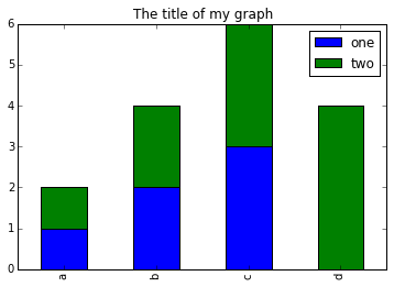
- You can use the
.unstack()method to transform grouped data into columns for each plotting. Try running.unstack()on some DataFrames above and see what it yields.
Start by transforming the grouped data into an unstacked layout, then create a stacked plot.
First we group data by language_code and then by is_dei.
PYTHON
# Step 1: Aggregate total checkouts per language_code regardless of is_dei
total_checkouts_per_language = works_df.groupby('language_code')['checkouts'].sum()

# Step 2: Sort these totals and get the top 10 language codes
top_10_languages = total_checkouts_per_language.sort_values(ascending=False).head(10).index

# Step 3: Filter the original DataFrame to include only these top 10 languages
filtered_df = works_df[works_df['language_code'].isin(top_10_languages)]

# Step 4: Group by both language_code and is_dei, and sum the checkouts
grouping = filtered_df.groupby(['language_code', 'is_dei'])['checkouts'].sum()
The last lines above calculates the sum of checkouts, for each language_code further broken down by DEI boolean flag, as a table and keeps only the top 10 most checked out items.
OUTPUT
language_code  is_dei
chi            False        7
               True         7
eng            False     4441
               True      2530
fre            False       70
               True        62
ger            False        7
               True         6
heb            False        6
               True         6
ita            False       21
               True         2
jpn            False       20
               True        20
kor            False        3
               True         3
per            False       27
               True        26
spa            False       95
               True        92
Name: checkouts, dtype: int64
After that, we use the .unstack() function on our
grouped data to figure out the total contribution of DEI verse non-DEI
for each language_code, and then plot the data.