Content from Short Introduction to Programming in Python

---

Last updated on 2024-05-13 | Edit this page

Estimated time: 30 minutes

Overview

Questions

• What is Python?
• Why should I learn Python?

Objectives

• Describe the advantages of using programming vs. completing repetitive tasks by hand.
• Define the following data types in Python: strings, integers, and floats.
• Perform mathematical operations in Python using basic operators.
• Define the following as it relates to Python: lists, tuples, and dictionaries.

The Basics of Python

---

Python is a general purpose programming language that supports rapid development of scripts and applications.

Python’s main advantages:

• Open Source software, supported by Python Software Foundation
• Available on all platforms
• It is a general-purpose programming language
• Supports multiple programming paradigms
• Very large community with a rich ecosystem of third-party packages

Interpreter

---

Python is an interpreted language which can be used in multiple ways:

• “Interactive” Mode: It functions like an “advanced calculator” Executing one command at a time:

PYTHON

user:host:~$ python
Python 3.5.1 (default, Oct 23 2015, 18:05:06)
[GCC 4.8.3] on linux2
Type "help", "copyright", "credits" or "license" for more information.
>>> 2 + 2
4
>>> print("Hello World")
Hello World

• “Scripting” Mode: Executing a series of “commands” saved in text file, usually with a .py extension after the name of your file:

BASH

user:host:~$ python my_script.py
Hello World

• “Cell” Mode: Commands are stored in specially formatted and interpreted files that contain independent cells that can be run seperately in any order we choose. The Scripting and Interactive modes are native to python and always available with any installation. Cell mode, on the other hand, requires software seperate from python itself like JupyterLab or VS Code with extensions. We will begin using Cell mode shortly after a few more examples using the built in modes.

Introduction to Python built-in data types

---

Strings, integers and floats

Python has built-in numeric types for integers, floats, and complex numbers. Strings are a built-in textual type.:

PYTHON

>>>text = "Data Carpentry"
>>> number = 42
>>> pi_value = 3.1415

Here we’ve assigned data to variables, namely text, number and pi_value, using the assignment operator =. The variable called text is a string which means it can contain letters and numbers. Notice that in order to define a string you need to have quotes around your text. To print out the value stored in a variable we can simply type the name of the variable into the interpreter:

PYTHON

>>> text
"Data Carpentry"

However, in a script, a print function is needed to output the text:

example.py

PYTHON

# A Python script file
# Comments in Python start with #
# The next line uses the print function to print out the text string
text = "Data Carpentry"
number = 42
pi_value = 3.1415
print(text)

Running the script

BASH

$ python example.py
Data Carpentry

Tip: The print function is a built-in function in Python. Later in this lesson, we will introduce methods and user-defined functions. The Python documentation is excellent for reference on the differences between them.

Operators

We can perform mathematical calculations in Python using the basic operators +, -, /, *, %:

PYTHON

>>> 2 + 2   #  addition
4
>>> 6 * 7   #  multiplication
42
>>> 2 ** 16  # power
65536
>>> 13 % 5  # modulo
3

We can also use comparison and logic operators: <, >, ==, !=, <=, >= and statements of identity such as and, or, not. The data type returned by this is called a boolean.

PYTHON

>>> 3 > 4
False
>>> True and True
True
>>> True or False
True

Sequential types: Lists and Tuples

---

Lists

Lists are a common data structure to hold an ordered sequence of elements. Each element can be accessed by an index. Note that Python indexes start with 0 instead of 1:

PYTHON

>>> numbers = [1, 2, 3]
>>> numbers[0]
1

A for loop can be used to access the elements in a list or other Python data structure one at a time:

PYTHON

>>> for num in numbers:
...     print(num)
...
1
2
3
>>>

Indentation is very important in Python. Note that the second line in the example above is indented. Just like three chevrons >>> indicate an interactive prompt in Python, the three dots ... are Python’s prompt for multiple lines. This is Python’s way of marking a block of code. [Note: you do not type >>> or ....]

To add elements to the end of a list, we can use the append method. Methods are a way to interact with an object (a list, for example). We can invoke a method using the dot . followed by the method name and a list of arguments in parentheses. Let’s look at an example using append:

PYTHON

>>> numbers.append(4)
>>> print(numbers)
[1, 2, 3, 4]
>>>

To find out what methods are available for an object, we can use the built-in help command:

PYTHON

help(numbers)

Help on list object:

class list(object)
 |  list() -> new empty list
 |  list(iterable) -> new list initialized from iterable's items
 ...

Tuples

A tuple is similar to a list in that it’s an ordered sequence of elements. However, tuples can not be changed once created (they are “immutable”). Tuples are created by placing comma-separated values inside parentheses ().

PYTHON

# tuples use parentheses
a_tuple= (1, 2, 3)
another_tuple = ('blue', 'green', 'red')
# Note: lists use square brackets
a_list = [1, 2, 3]

Challenge - Tuples

1. What happens when you type a_tuple[2]=5 vs a_list[1]=5 ?
2. Type type(a_tuple) into python - what is the object type?

Show me the solution

1. As a tuple is immutable, it does not support item assignment. Elements in a list can be altered individually.

2. tuple

Dictionaries

---

A dictionary is a container that holds pairs of objects - keys and values.

PYTHON

>>> translation = {'one': 1, 'two': 2}
>>> translation['one']
1

Dictionaries work a lot like lists - except that you index them with keys. You can think about a key as a name for or a unique identifier for a set of values in the dictionary. Keys can only have particular types - they have to be “hashable”. Strings and numeric types are acceptable, but lists aren’t.

PYTHON

>>> rev = {1: 'one', 2: 'two'}
>>> rev[1]
'one'
>>> bad = {[1, 2, 3]: 3}
Traceback (most recent call last):
  File "<stdin>", line 1, in <module>
TypeError: unhashable type: 'list'

In Python, a “Traceback” is an multi-line error block printed out for the user.

To add an item to the dictionary we assign a value to a new key:

PYTHON

>>> rev = {1: 'one', 2: 'two'}
>>> rev[3] = 'three'
>>> rev
{1: 'one', 2: 'two', 3: 'three'}

Using for loops with dictionaries is a little more complicated. We can do this in two ways:

PYTHON

>>> for key, value in rev.items():
...     print(key, '->', value)
...
1 -> one
2 -> two
3 -> three

or

PYTHON

>>> for key in rev.keys():
...     print(key, '->', rev[key])
...
1 -> one
2 -> two
3 -> three
>>>

Challenge - Can you do reassignment in a dictionary?

1. First check what rev is right now (remember rev is the name of our dictionary).

Type:

PYTHON

>>> rev

2. Try to reassign the second value (in the key value pair) so that it no longer reads “two” but instead reads “apple-sauce”.

3. Now display rev again to see if it has changed.

Show me the solution

You should see the following output: {1: 'one', 2: 'two', 3: 'three'}

PYTHON

rev[2] = "apple-sauce"

PYTHON

{1: 'one', 2: 'apple-sauce', 3: 'three'}

Dictionaries as of python 3.7 are now in inserstion order be default. Anything you see talking about dictionaries beying unordered can be safely ignored as long as you are using python 3.7 or later.

Functions

---

While functions work just fine in all three modes, let’s open JupyterLab so we can use cell mode moving forward with the rest of the workshop for the sake of convenience. Let’s do that from our terminal where in order to save time in the next episode, we will launch JupyterLab with the workshop directory containing our data files as the working directory.

Opening JupyterLab

BASH

# navigate to or start your terminal from the worskhop directory
$ jupyter lab
# you may see various status messages as it spins up jupyter server and launches your default browser

Defining a section of code as a function in Python is done using the def keyword. For example a function that takes two arguments and returns their sum can be defined as:

PYTHON

def add_function(a, b):
    result = a + b
    return result

z = add_function(20, 22)
print(z)
42

Key points about functions are:

• definition starts with def
• function body is indented
• return keyword precedes returned value

Content from Starting With Data

---

Last updated on 2024-06-18 | Edit this page

Estimated time: 60 minutes

Overview

Questions

• How can I import data in Python?
• What is Pandas?
• Why should I use Pandas to work with data?

Objectives

• Navigate the workshop directory and download a dataset.
• Explain what a library is and what libraries are used for.
• Describe what the Python Data Analysis Library (Pandas) is.
• Load the Python Data Analysis Library (Pandas).
• Use read_csv to read tabular data into Python.
• Describe what a DataFrame is in Python.
• Access and summarize data stored in a DataFrame.
• Define indexing as it relates to data structures.
• Perform basic mathematical operations and summary statistics on data in a Pandas DataFrame.
• Create simple plots.

Working With Pandas DataFrames in Python

---

We can automate the processes listed above using Python. It is efficient to spend time building code to perform these tasks because once it is built, we can use our code over and over on different datasets that share a similar format. This makes our methods easily reproducible. We can also share our code with colleagues so they can replicate our analysis.

Starting in the same spot

If you do not already have JupyterLab opened from the workshop directroy, let’s do that now. Doing so should help us avoid path and file name issues. At this time please navigate to the workshop directory in your terminal.

Opening JupyterLab

BASH

# navigate to or start your terminal from the worskhop directory
$ jupyter lab
# you may see various status messages as it spins up jupyter server 
# and launches your default browser

A quick aside that there are Python libraries like OS Library that can work with our directory structure, however, that is not our focus today.

Alex: our user story

Alex is a researcher interested in exploring the collection of fictional works at their university and assessing how representative it is in relation to the student body. Alex was able to find a pre-liminary dataset assembled by a previous researcher from which they want to create some exploratory plots and intermediate datasets in order to determine next steps to expand on this line of inquiry.

Alex could do some of this work using spreadsheet systems but this can be time consuming to do and lead to mistakes that are hard to detect.

This workshop will show how Python can be used to automate some of the processes allowing them to be re-run in the future.

Our Data

We will be using files from the data folder. This section will use the all_works.csv file that can be found in your data folder.

The dataset is stored as a comma separated (.csv) file, where each row holds information for a single title, and the columns represent diferent aspects (variables) of each entry:

Column	Description
title	Title of Work
subjects	List of Subjects
mms_id	Metadata Management System ID
author	Author(s) delimited with ‘;’
publication_date	Year of Publication
publication_place	Place of Publication
language_code	Language of Text
resource_type	Type of resource, e.g. physical, electronic
acquisition_date	Date of Acquisition
is_dei	Boolean for whether work meets broadest definition of a DEI work
checkouts	Count of number of times

Semantics of DEI

• Diversity, Equity and Inclusion are not concrete terms that can be divorced from history and geography. Thus, it is incumbent on academic researchers to define what that means in their practice.
  
• Arguably, any resource is potentially useful in the pursuit of DEI research if for no other reason as to provide contrast and foreground for other works, so designating something a DEI resource will always be a judgment call.
  
• Here, though, the is_dei flag is applied to any works with subjects deemed outside those with a male, western European lineage. That determination is also a judgment call on multiple levels that you may disagree with, and that is okay. Not only might you disagree with what subjects do or do not share a male, western European lineage, but we are also at the mercy of the cataloger wrestling with their own biases while applying a limited scope of slowly evolving options.
• Our flag will never be perfect, so our goal should be good enough with the time and information we have. You can spot check the subjects deemed dei and non-dei.
• All datasets should be approached with a sceptical eye. When we are done here, you should not only know how to leverage datasets, but interogate and adjust them to adhere to different assumptions. Just be sure to make those adjustments and assumptions clear to those who follow after you.

If we open the all_works.csv data file using a text editor, the first few rows of our first file look like this:

title,subjects,mms_id,author,publication_date,publication_place,language_code,resource_type,acquisition_date,is_dei,subject_count,chekcouts
"""A god of justice?"" : the problem of evil in twentieth-century Black literature","['American literature--African American authors--History and criticism', 'African Americans--Intellectual life--20th century', 'African Americans--Intellectual lif', 'American literature--African American author']",991004617919702908,"Whitted, Qiana J., 1974-",2009.0,Charlottesville,eng,Book - Physical,2016-06-26 23:51:01,True,4,
"""Baad bitches"" and sassy supermamas : Black power action films","['Blaxploitation films--United States--History and criticism', 'African American women heroes in motion pictures', 'African American women heroes in motion picture', 'Blaxploitation film', 'Blaxploitation Film']",991003607949702908,"Dunn, Stephane, 1967-",2008.0,Urbana,eng,Book - Physical,2011-12-13 03:51:20,True,5,1.0
"""Codependent lesbian space alien seeks same""","['Lesbians--Drama', 'Lesbians', 'Video recordings for the hearing impaired']",991013190057102908,"Olnek, Madeleine.; Space Aliens, LLC.",2011.0,"[New York, NY?]",eng,Projected medium - Physical,2016-11-10 07:56:09,True,3,1.0
"""Lactilla tends her fav'rite cow"" : ecocritical readings of animals and women in eighteenth-century British labouring-class women's poetry","['English poetry--Women authors--History and criticism', 'Working class writings, English--History and criticism', 'Ecofeminism in literature', 'English poetry--Women authors', 'Working class women in literature', 'Working class writings, English']",991003662979702908,"Milne, Anne.",2008.0,Lewisburg,eng,Book - Physical,2015-10-07 16:31:28,True,8,

Why software libraries

Theoretically, you could use only built in python functions to interact directly with the text file, but you would be re-inventing the wheel. Better to do a little research and find someone who has already grappled with similar problems and stand on their shoulders instead. Programming often has a mechanism to facilitate this. In python, the are called libraries.

A library in Python contains a set of tools (functions) that perform different actions. Importing a library is like getting a set of particular tools out of a storage locker and setting them up on the bench for use in a project. Once a library is set up, its functions can be used or called to perform different tasks.

Why Pandas in Python

One of the best options for working with tabular data in Python is to use the Python Data Analysis Library (a.k.a. Pandas Library). The Pandas library provides structures to sort our data, can produce high quality plots in conjunction with other libraries such as matplotlib, and integrates nicely with libraries that use NumPy (which is another common Python library) arrays.

Loading a library

Python doesn’t load all of the libraries available to it by default. We have to add an import statement to our code in order to use library functions required for our project. To import a library, we use the syntax import libraryName, where libraryName represents the name of the specific library we want to use. Note that the import command calls a library that has been installed previously in our system. If we use the import command to call for a library that does not exist in our local system, the command will throw and error when executed. In this case, you can use pip command in another terminal window to install the missing libraries. See here for details on how to do this.

Moreover, if we want to give the library a nickname to shorten the command, we can add as nickNameHere. An example of importing the pandas library using the common nickname pd is:

PYTHON

import pandas as pd

Each time we call a function that’s in a library, we use the syntax LibraryName.FunctionName. Adding the library name with a . before the function name tells Python where to find the function. In the example above, we have imported Pandas as pd. This means we don’t have to type out pandas each time we call a Pandas function.

Reading CSV Data Using Pandas

---

We will begin by locating and reading in a data which in CSV format. We can use Pandas’ read_csv function to pull either a local (a file in our machine) or a remote (one that is available for downloading from the web) file into a Pandas table or DataFrame.

In order to read data in, we need to know where the data is stored on our computer or its URL address if the file is available on the web.

PYTHON

# note that pd.read_csv is used because we imported pandas as pd
# note that this assumes that the data file is in the same location
# as the Jupyter notebook to simplify pathing
pd.read_csv("all_works.csv")

So What’s a DataFrame?

A DataFrame is a 2-dimensional data structure that can store data of different types (including characters, integers, floating point values, factors and more) in columns. It is similar to a spreadsheet or a data.frame in R. A DataFrame always has an index (0-based integers by default). An index refers to the position of an element in the data structure.

The above command yields the output similar to below, but formatted differently

                                                   title                                           subjects  ...  is_dei checkouts
0      "A god of justice?" : the problem of evil in t...  ['American literature--African American author...  ...    True         0
1      "Baad bitches" and sassy supermamas : Black po...  ['Blaxploitation films--United States--History...  ...    True         1
2           "Codependent lesbian space alien seeks same"  ['Lesbians--Drama', 'Lesbians', 'Video recordi...  ...    True         1
3      "Lactilla tends her fav'rite cow" : ecocritica...  ['English poetry--Women authors--History and c...  ...    True         0
4      "The useless mouths", and other literary writings  ['French drama--20th century--Translations int...  ...    True         1
...                                                  ...                                                ...  ...     ...       ...
14227  ¡Ban c/s this! : the BSP anthology of Xican@ l...  ["Littérature américaine--Auteurs américain...  ...   False         0
14228  ¡Muy pop! : conversations on Latino popular cu...  ['Popular culture--United States', "Littératu...  ...   False         1
14229  ¡Viva la historieta! : Mexican comics, NAFTA, ...  ['Mondialisation dans la littérature', "Mondi...  ...   False         0
14230                 Đời về cơ bản là buồn cười  ['Life--Comic books, strips, etc', 'Life', 'Co...  ...   False         3
14231  Đường vào văn chương : phê bình lý trí ...  ['Literature, Modern--History and criticism--T...  ...   False         0

[14232 rows x 11 columns]

We can see that there were 14232 rows parsed. Each row has 11 columns. The first column displayed is the index of the DataFrame. The index is used to identify the position of the data, but it is not an actual column of the DataFrame. It looks like the read_csv function in Pandas read our file properly. However, we haven’t saved any data to memory so we can not work with it yet. We need to assign the DataFrame to a variable so we can call and use the data. Remember that a variable is a name given to a value, such as x, or data. We can create a new object with a variable name by assigning a value to it using =.

Let’s call the imported data works_df:

PYTHON

works_df = pd.read_csv("all_works.csv")

Notice that when you assign the imported DataFrame to a variable, Python does not produce any output on the screen. We can print the value of the works_df object by typing its name into the cell and running it. If you were doing this in a script file, you would need to use print(works_df). Not needing to do so here is another convenience feature of Jupyter.

PYTHON

works_df

which prints contents like above

Exploring our Data

We can use attributes and methods provided by the DataFrame object to summarize and access the data stored in it.

Attributes are called by using the syntax df_object.attribute. For example, we can use the dtypes attribute of the DataFrame to return a Series object of the dataypes for each column in the DataFrame.

works_df.dtypes

which returns output similar to:

title                object
subjects             object
mms_id                int64
author               object
publication_date      int64
publication_place    object
language_code        object
resource_type        object
acquisition_date     object
is_dei                 bool
checkouts             int64
dtype: object

int64 represents numeric integer values - int64 cells cannot store decimals. object represents strings (letters and numbers). float64 represents numbers with decimals.

Methods are called by using the syntax df_object.method(). Note the inclusion of open brackets at the end of the method. Python treats methods as functions associated with a dataframe rather than just a property of the object as with attributes. Similarly to functions, methods can include optional parameters inside the brackets to change their default behaviour.

As an example, works_df.head() gets the first few rows in the DataFrame works_df using the head() method. With a method, we can supply extra information within the open brackets to control its behaviour, e.g. works_df.head(25).

Let’s try out a few of the common DataFrame methods and attributes.

Challenge - DataFrames

Using our DataFrame works_df, try out the attributes & methods below to see what they return.

1. works_df.columns

2. works_df.shape Take note of the output of shape - what format does it return the shape of the DataFrame in?

HINT: More on tuples, here.

3. works_df.head() Also, what does works_df.head(15) do?

4. works_df.tail()

5. works_df.info()

Show me the solution

1. works_df.columns return list of column as a data type pandas.core.indexes.base.Index

2. works_df.shape. Take note of the output of the shape method. What format does it return the shape of the DataFrame in?

type(works_df.shape) -> Tuple, (rows, columns), i.e. standard row-first Python format

3. works_df.head(). Also, what does works_df.head(15) do?

Show first N lines

4. works_df.tail()

Show last N lines

5. works_df.info() returns a table with wealth of information about number of colums, datatypes, missing values, memory usage.

Summary Statistics & Groups in Pandas

We often want to calculate summary statistics for our data. This can be useful even at the exploratory phase as it can help you understand the ranges of your data and detect possible outliers.

We can calculate basic statistics for all records in a single column using the syntax below:

PYTHON

works_df['checkouts'].describe()

gives output

PYTHON

count    14232.000000
mean         0.526349
std          1.432189
min          0.000000
25%          0.000000
50%          0.000000
75%          1.000000
max         43.000000
Name: checkouts, dtype: float64

We can also extract specific metrics for one or various columns if we wish:

PYTHON

works_df['checkouts'].min()
works_df['checkouts'].max()
works_df['checkouts'].mean()
works_df['checkouts'].std()
works_df['checkouts'].count()

But if we want to summarize by one or more variables, for example checkouts by language_code, we can use the .groupby method. When executed, this method creates a DataFrameGroupBy object containing a subset of the original DataFrame. Once we’ve created it, we can quickly calculate summary statistics by a group of our choice. For example the following code will group our data by language_code.

PYTHON

# Group data by status
grouped_data = works_df.groupby('language_code')

If we execute the pandas function describe on this new object we will obtain descriptive stats for all the numerical columns in works_df grouped by the different cities available in the publication_place column of the DataFrame.

PYTHON

# summary statistics for all numeric columns by place
grouped_data.describe()
# provide the mean for each numeric column by place
grouped_data.mean()

grouped_data.mean(numeric_only=True) OUTPUT:

PYTHON

	mms_id	publication_date	is_dei	checkouts
language_code				
ara	9.910032e+17	2009.000000	0.400000	0.000000
bos	9.910132e+17	2018.000000	0.500000	0.000000
cat	9.910131e+17	2011.000000	0.500000	0.000000
chi	9.910073e+17	2011.400000	0.500000	0.700000
# Truncated for brevity

The groupby command is powerful in that it allows us to quickly generate summary stats, but how do you know what columns will make good group by candidates.

Let’s use the publication locations as an example by finding out how many unique values are in that column. DataFrames and Series object often share methods allowing for two different approaches. One method calls pd.unique function directly off the dataframe and passes in the column of intrest. In the other, we can a method directly off the column works_df['publication_place'].unique(). The output is identical listing the unique values in the publication_place column.

PYTHON

pd.unique(works_df['publication_place'])

PYTHON

works_df['publication_place'].unique()

either returns:

PYTHON

array(['Charlottesville', 'Urbana', '[New York, NY?]', ...,
       'Cambridge [UK] ; Medford', 'Arles', '[London]:'], dtype=object)

Challenge - Statistics

1. Create a list of unique publicaton years found in the data. Call it years. How many unique years are there in the data?

2. What is the difference between len(years) and works_df['publication_date'].nunique()?

Show me the solution

1. Create a list of unique locations found in the index data. Call it places. How many unique location are there in the data?

PYTHON

years = pd.unique(works_df["publication_date"])
len(years)

2. What is the difference between len(years) and works_df["publication_date"].nunique()?

Both do result in the same output, making it alternative ways of getting the unique values. nunique combines the count and unique value extraction.

Challenge - Summary Data

1. Create your own groupy object based on publicatin_place and take the mean of checkouts.
2. What is the mean number of checkout for works published in [Washington, D.C.].
3. What does the summary stats uncover about the quality of data in the publication_place column?
4. What happens when you group by two columns using the following syntax and then grab mean values:

PYTHON

grouped_data2 = all_works_df.groupby(['resource_type', 'language_code'])
mean_values_by_type_and_language = grouped_data2.mean(numeric_only=True)
mean_values_by_type_and_language

Show me the solution

PYTHON

grouped_data = all_works_df.groupby('publication_place')
means_by_publication_place = grouped_data.mean(numeric_only=True)
means_by_publication_place['checkouts']

2. We can see in the list that is 0.000000.
3. We can see that the entries vary in how they are formatted. For a real analysis, you would likley want to clean this up before proceeding. We can browse the full list using code like the following to confirm:

PYTHON

for place in sorted(all_works_df['publication_place'].unique()):
    print(place)

4. This code will create a GroupBy object grouped by both resource_type and language_code and then calculate the mean of all numerical columns within each group. This is useful for seeing trends across different types of resources and languages, potentially revealing interactions between these categories.

Quickly Creating Summary Counts in Pandas

Let’s next count the number of publications for each author(s). We can do this in a few ways, but we’ll use groupby combined with a count() method.

PYTHON

# count the number of texts by authors / groups of authors
author_counts = works_df.groupby('author')['mms_id'].count()
author_counts

Or, we can also count just the rows that have the a specifig author like “Abate, Michelle Ann, 1975-”:

PYTHON

author_counts = works_df.groupby('author')['mms_id'].count()['Abate, Michelle Ann, 1975-']
author_counts

How does the code work? works_df.groupby('author')['mms_id'].count() actually returns a series where author is the index. We then filter by that specific index.

Just because you can doesn’t mean you should

Many of our works have groups of authors, and they are all contained in a single cell. This makes some questions easier to ask and some harder. It is actually non-trivial to get a count of all of “Abate, Michelle Ann, 1975-” works since she may be listed among other author groups. Thus grouping by author and filtering on this key given the current data configuration may not be telling us what we thought it was. Thus it is important to know your data well and format it and reformat it to meet your analysis needs. You need to stay vigilant and check your understanding. Python won’t stop you from doing a poor analysis very efficiently.

Math Operations

If we wanted to, we could perform math on an entire numerical column of our data. To demonstrate this, let’s add another column that shows the percentage of total checkouts for each work.

PYTHON

all_checkouts = works_df.checkouts.sum()
# because "checkout_percentage" is not in our columns index, pandas add is as a new column.
works_df["checkout_percentage"] = (works_df.checkouts / all_checkouts) * 100
works_df.checkout_percentage

Quick & Easy Plotting Data Using Pandas

---

We will looks at plotting more in depth later, but we can rapidly plot our summary stats using Pandas.

PYTHON

# group data
is_dei_count = works_df.groupby("is_dei")["mms_id"].count() 
# set equal to variable so we can set additional parameters
plot = is_dei_count.plot(kind="bar", title="Checkout by DEI Status")
#lablel the y-axis
plot.set_ylabel("Checkouts")

What does this graph show? Let’s step through

• works_df.groupby("is_dei") : This groups the works by the boolean flag.

• works_df.groupby("is_dei")["mms_id"] : This chooses a single column to count, rather than counting all columns since we only want one number to plot. You could effectively pick any column.

• works_df.groupby("is_dei")["mms_id"].count() : this counts the instances, i.e. how many works per given boolean value?

• plot = is_dei_count.plot(kind="bar",title="Checkout by DEI Status") : this plots a bar chart with the boolean flag on x axis and count on the y axis, sets title.

• plot.set_ylabel("Checkouts") : this labels the y-axis

Challenge

Summary Plotting Challenge

Create a stacked bar plot, showing the checkouts, per language_code, with the is_dei stacked on top of each other for the 10 languages with the most checkouts. Drop any records where is_dei True column is NAN. The language_code should go on the X axis, and the checkouts on the Y axis. Some tips are below to help you solve this challenge:

• For more on Pandas plots, visit this link.
• You can use the code that follows to create a stacked bar plot but the data to stack need to be in individual columns. Here’s a simple example with some data where ‘a’, ‘b’, and ‘c’ are the groups, and ‘one’ and ‘two’ are the subgroups.

d = {'one' : pd.Series([1., 2., 3.], index=['a', 'b', 'c']),'two' : pd.Series([1., 2., 3., 4.], index=['a', 'b', 'c', 'd'])}
pd.DataFrame(d)

shows the following data

      one  two
  a    1    1
  b    2    2
  c    3    3
  d  NaN    4

We can plot the above with

# plot stacked data so columns 'one' and 'two' are stacked
my_df = pd.DataFrame(d)
my_df.plot(kind='bar', stacked=True, title="The title of my graph")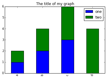

Stacked Bar Plot

• You can use the .unstack() method to transform grouped data into columns for each plotting. Try running .unstack() on some DataFrames above and see what it yields.

Start by transforming the grouped data into an unstacked layout, then create a stacked plot.

Show me the solution

First we group data by language_code and then by is_dei.

PYTHON

# Step 1: Aggregate total checkouts per language_code regardless of is_dei
total_checkouts_per_language = works_df.groupby('language_code')['checkouts'].sum()

# Step 2: Sort these totals and get the top 10 language codes
top_10_languages = total_checkouts_per_language.sort_values(ascending=False).head(10).index

# Step 3: Filter the original DataFrame to include only these top 10 languages
filtered_df = works_df[works_df['language_code'].isin(top_10_languages)]

# Step 4: Group by both language_code and is_dei, and sum the checkouts
grouping = filtered_df.groupby(['language_code', 'is_dei'])['checkouts'].sum()

The last lines above calculates the sum of checkouts, for each language_code further broken down by DEI boolean flag, as a table and keeps only the top 10 most checked out items.

OUTPUT

language_code  is_dei
chi            False        7
               True         7
eng            False     4441
               True      2530
fre            False       70
               True        62
ger            False        7
               True         6
heb            False        6
               True         6
ita            False       21
               True         2
jpn            False       20
               True        20
kor            False        3
               True         3
per            False       27
               True        26
spa            False       95
               True        92
Name: checkouts, dtype: int64

After that, we use the .unstack() function on our grouped data to figure out the total contribution of DEI verse non-DEI for each language_code, and then plot the data.

PYTHON

# Step 5: Unstack the is_dei level for plotting
grouping_unstacked = grouping.unstack()

# Plot the data
plot = grouping_unstacked.plot(kind="bar", stacked=True, title="DEI Checkouts By Language", figsize=(10, 5), logy=True)
plot.set_ylabel("Checkouts")

Content from Indexing, Slicing and Subsetting DataFrames in Python

---

Last updated on 2024-06-18 | Edit this page

Estimated time: 60 minutes

Overview

Questions

• How can I access specific data within my data set?
• How can Python and Pandas help me to analyse my data?

Objectives

• Describe what 0-based indexing is.
• Manipulate and extract data using column headings and index locations.
• Employ slicing to select sets of data from a DataFrame.
• Employ label and integer-based indexing to select ranges of data in a dataframe.
• Reassign values within subsets of a DataFrame.
• Create a copy of a DataFrame.
• Query /select a subset of data using a set of criteria using the following operators: =, !=, >, <, >=, <=.
• Locate subsets of data using masks.
• Describe BOOLEAN objects in Python and manipulate data using BOOLEANs.

In lesson 01, we read a CSV into a Python pandas DataFrame. We learned:

• how to save the DataFrame to a named object,
• how to perform basic math on the data,
• how to calculate summary statistics, and
• how to create plots of the data.

In this lesson, we will explore ways to access different parts of the data using:

• indexing,
• slicing, and
• subsetting.

Loading our data

---

We will continue to use the works dataset that we worked with in the last lesson. Let’s reopen and read in the data again:

PYTHON

# Make sure pandas is loaded
import pandas as pd

# read in the survey csv
works_df = pd.read_csv("all_works.csv")

Indexing and Slicing in Python

---

We often want to work with subsets of a DataFrame object. There are different ways to accomplish this including: using labels (column headings), numeric ranges, or specific x,y index locations.

Selecting data using Labels (Column Headings)

---

We use square brackets [] to select a subset of an Python object. As we saw in the previous espisode, we can select all data from the column named checkouts from the works_df DataFrame by name. There are two ways to do this:

PYTHON

# Method 1: select a 'subset' of the data using the column name
works_df['checkouts']

# Method 2: use the column name as an 'attribute'; gives the same output
works_df.checkouts

We can also create a new object that contains only the data within the checkouts column as follows:

PYTHON

# creates an object, checkouts_series, that only contains the `checkouts` column
checkouts_series = works_df['checkouts']

We can pass a list of column names too, as an index to select columns in that order. This is useful when we need to reorganize our data.

NOTE: If a column name is not contained in the DataFrame, an exception (error) will be raised.

PYTHON

# select the title and checkouts columns from the DataFrame
works_df[['title', 'checkouts']]

# what happens when you flip the order?
works_df[['checkouts', 'title']]

#what happens if you ask for a column that doesn't exist?
works_df['Texts']

Extracting Range based Subsets: Slicing

---

REMINDER: Python Uses 0-based Indexing

Let’s remind ourselves that Python uses 0-based indexing. This means that the first element in an object is located at position 0. This is different from other tools like R and Matlab that index elements within objects starting at 1.

PYTHON

# Create a list of numbers:
a = [1, 2, 3, 4, 5]

Challenge - Extracting data

1. What value does the code below return?

PYTHON

a[0]

2. How about this:

PYTHON

a[5]

3. In the example above, calling a[5] returns an error. Why is that?

4. What about?

PYTHON

a[len(a)]

Show me the solution

• What value does the code below return? a[0]

  1, as Python starts with element 0 (for Matlab users: this is different!)

• How about this: a[5]

  IndexError

• In the example above, calling a[5] returns an error. Why is that?

  The list has no element with index 5 (going from 0 till 4).

• What about? a[len(a)]

  IndexError

Slicing Subsets of Rows in Python

---

Slicing using the [] operator selects a set of rows and/or columns from a DataFrame. To slice out a set of rows, you use the following syntax: data[start:stop]. When slicing in pandas the start bound is included in the output. The stop bound should be set to one step BEYOND the row you want to select. So if you want to select rows 0, 1 and 2 your code would look like this:

PYTHON

# select rows 0, 1, 2 (row 3 is not selected)
works_df[0:3]

The stop bound in Python is different from what you might be used to in languages like Matlab and R.

PYTHON

# select the first 5 rows (rows 0, 1, 2, 3, 4)
works_df[:5]

# select the last element in the list
# (the slice starts at the last element,
# and ends at the end of the list)
works_df[-1:]

We can also reassign values within subsets of our DataFrame.

But before we do that, let’s look at the difference between the concept of copying objects and the concept of referencing objects in Python.

Copying Objects vs Referencing Objects in Python

---

Let’s start with an example:

PYTHON

# using the 'copy() method'
true_copy_works_df = works_df.copy()

# using '=' operator
ref_works_df = works_df

You might think that the code ref_works_df = works_df creates a fresh distinct copy of the works_df DataFrame object. However, using the = operator in the simple statement y = x does not create a copy of our DataFrame. Instead, y = x creates a new variable y that references the same object that x refers to. To state this another way, there is only one object (the DataFrame), and both x and y refer to it.

In contrast, the copy() method for a DataFrame creates a true copy of the DataFrame.

Let’s look at what happens when we reassign the values within a subset of the DataFrame that references another DataFrame object:

 # Assign the value `0` to the first three rows of data in the DataFrame
 ref_works_df[0:3] = 0
 ```

Let's try the following code:

 ```
# ref_works_df was created using the '=' operator
 ref_works_df.head()

 # works_df is the original dataframe
 works_df.head()

What is the difference between these two dataframes?

When we assigned the first 3 columns the value of 0 using the ref_works_df DataFrame, the works_df DataFrame is modified too. Remember we created the reference ref_survey_df object above when we did ref_survey_df = works_df. Remember works_df and ref_works_df refer to the same exact DataFrame object. If either one changes the object, the other will see the same changes to the reference object.

To review and recap:

• Copy uses the dataframe’s copy() method

  true_copy_works_df = works_df.copy()

• A Reference is created using the = operator

  PYTHON

  ref_works_df = works_df

Okay, that’s enough of that. Let’s create a brand new clean dataframe from the original data CSV file.

PYTHON

works_df = pd.read_csv("all_works.csv")

Slicing Subsets of Rows and Columns in Python

---

We can select specific ranges of our data in both the row and column directions using either label or integer-based indexing. Columns can be selected either by their name, or by the index of their location in the dataframe. Rows can only be selected by their index, but the index is not necessarily an integer as it is by default.

• loc is primarily label based indexing. Integers may be used but they are interpreted as a label.
• iloc is primarily integer based indexing

iloc

To select a subset of rows and columns from our DataFrame, we can use the iloc method. For example, we can select subjects, mms_id, and author (columns 2, 3 and 4 if we start counting at 1), like this:

PYTHON

# iloc[row slicing, column slicing]
works_df.iloc[0:3, 1:4]

which gives the output

	                                      subjects	              mms_id	                 author
0	['American literature--African American author...	991004617919702908	Whitted, Qiana J., 1974-
1	['Blaxploitation films--United States--History...	991003607949702908	Dunn, Stephane, 1967-
2	['Lesbians--Drama', 'Lesbians', 'Video recordi...	991013190057102908	Olnek, Madeleine.; Space Aliens, LLC.

Notice that we asked for a slice from 0:3. This yielded 3 rows of data. When you ask for 0:3, you are actually telling Python to start at index 0 and select rows 0, 1, 2 up to but not including 3.

We can also select a specific data value using a row and column location within the DataFrame and iloc indexing:

PYTHON

# Syntax for iloc indexing to finding a specific data element
dat.iloc[row, column]

In this iloc example,

PYTHON

works_df.iloc[2, 6]

gives the output

'eng'

Remember that Python indexing begins at 0. So, the index location [2, 6] selects the element that is 3 rows down and 7 columns over in the DataFrame.

loc

Let’s explore ways to index and select subsets of data with loc:

PYTHON

# select all columns for rows of index values 0 and 10
works_df.loc[[0, 10], :]

# what does this do?
works_df.loc[0, ['author', 'title', 'checkouts']]

# What happens when you type the code below?
works_df.loc[[0, 10, 149], :]

NOTE: Labels must be found in the DataFrame or you will get a KeyError.

Indexing by labels loc differs from indexing by integers iloc. With iloc, the start bound and the stop bound are inclusive. When using loc instead, integers can also be used, but the integers refer to the index label and not the position. For example, using loc and select 1:4 will get a different result than using iloc to select rows 1:4.

Challenge - Range

1. Given the three range indicies below, what do you expect to get back? Does it match what you actually get back?

• works_df[0:1]
• works_df[:4]
• works_df[:-1]

Suggestion: You can also select every Nth row: works_df[1:10:2]. So, how to interpret works_df[::-1]?

• What is the difference between works_df.iloc[0:4, 1:4] and works_df.loc[0:4, 1:4]?

Show me the solution

Checks the position, or the name. The second is like it would be in a dictionary, asking for the key-names. Column names 1:4 do not exist, resulting in an error. Check also the difference between works_df.loc[0:4] and works_df.iloc[0:4]

Subsetting Data using Criteria

---

A mask can be useful to locate where a particular subset of values exist or don’t exist. To understand masks, we also need to understand BOOLEAN objects in Python.

Boolean values include True or False. For example,

PYTHON

# set x to 5
x = 5

# what does the code below return?
x > 5

# how about this?
x == 5

When we ask Python what the value of x > 5 is, we get False. This is because the condition,x is not greater than 5, is not met since x is equal to 5.

To create a boolean mask:

• Set the True / False criteria (e.g. values > 5 = True)
• Python will then assess each value in the object to determine whether the value meets the criteria (True) or not (False).
• Python creates an output object that is the same shape as the original object, but with a True or False value for each index location.

Pandas provides multiple ways to to generate boolean sets of boolean criteria to use for filtering. For example, we can select all rows where subjects includes the work “Diversity” by using the contains method in the str namespace.

PYTHON

works_df.loc[works_df["subjects"].str.contains("Diversity", na=False)]

Or we can select all rows with a checkouts greater than 0:

PYTHON

works_df[works_df["checkouts"] > 0]

We can define sets of criteria too using & or |. Parenthesis are required to help with order of computation:

PYTHON

works_df[(works_df.publication_date >= 2010) & (works_df.publication_date <= 2015)]

Python Syntax Cheat Sheet

Use can use the syntax below when querying data by criteria from a DataFrame. Experiment with selecting various subsets of the “works” data.

• Equals: ==
• Not equals: !=
• Greater than, less than: > or <
• Greater than or equal to >=
• Less than or equal to <=

Challenge - Advanced Queries

1. Select a subset of rows in the works_df DataFrame that was published before 2010 and checked out less than five times. How many rows did you end up with? What did your neighbor get?

2. You can use the isin command in Python to query a DataFrame based upon a list of values as follows. Notice how the indexing relies on a reference to the dataframe being indexed. Think about the order in which the computer must evaluate these statements.

PYTHON

works_df[
        works_df['publication_date'].isin([listGoesHere])
        ]

Use the isin function to find all books published in either 2010 or 2015. How many are there?

3. Experiment with other queries. Create a query that finds all rows with a checkouts greater than or equal to 1.

4. The ~ symbol in Python can be used to return the OPPOSITE of the selection that you specify in Python. It is equivalent to is not in. Write a query that selects all rows with publication_date NOT equal to 2010 or 2015 in the works data.

Show me the solution

1. PYTHON

   works_df[(works_df.publication_date < 2010) & (works_df.checkouts < 5)]

2. PYTHON

   works_df[works_df['publication_date'].isin([2010,2015])]

PYTHON

works_df[works_df['checkouts']>=1]

PYTHON

works_df[~works_df['publication_date'].isin([2010,2015])]

Setting values using slicing by criteria

---

Using slicing by criteria, we can directly set values. For example, if we thought Abusive men–Drama was relevant to DEI, we could set the is_dei flag on all records where subject contained that string using the following syntax

PYTHON

works_df.loc[works_df.subjects.str.contains('Abusive men--Drama'), 'is_dei'] = True

Challenge - Adjusting the DEI flag

Create a true copy of the works_df. Find a subject value you would like to remove. If there is nothing you have issue with, just pick one at random.

Use those critera to change the is_dei flag in your true copy to False.

Show me the solution

For the example we will use “Aristocracy (Social class”

PYTHON

copy = works_df.copy()
# we have to escape the '(' symbol
copy.loc[works_df.subjects.str.contains('Aristocracy \(Social class'), 'is_dei'] = False

Content from Data Types and Formats

---

Last updated on 2024-05-16 | Edit this page

Estimated time: 45 minutes

Overview

Questions

• What types of data can be contained in a DataFrame?
• Why is the data type important?

Objectives

• Describe how information is stored in a Python DataFrame.
• Define the two main types of data in Python: text and numerics.
• Examine the structure of a DataFrame.
• Modify the format of values in a DataFrame.
• Describe how data types impact operations.
• Define, manipulate, and interconvert integers and floats in Python.
• Analyze datasets having missing/null values (NaN values).

The format of individual columns and rows will impact analysis performed on a dataset read into python. For example, you can’t perform mathematical calculations on a string (text formatted data). This might seem obvious, however sometimes numeric values are read into python as strings. In this situation, when you then try to perform calculations on the string-formatted numeric data, you get an error.

In this lesson we will review ways to explore and better understand the structure and format of our data.

Types of Data

---

How information is stored in a DataFrame or a python object affects what we can do with it and the outputs of calculations as well. There are two main types of data that we’re explore in this lesson: numeric and text data types.

Numeric Data Types

Numeric data types include integers and floats. A floating point (known as a float) number has decimal points even if that decimal point value is 0. For example: 1.13, 2.0 1234.345. If we have a column that contains both integers and floating point numbers, Pandas will assign the entire column to the float data type so the decimal points are not lost.

An integer will never have a decimal point. Thus if we wanted to store 1.13 as an integer it would be stored as 1. Similarly, 1234.345 would be stored as 1234. You will often see the data type Int64 in python which stands for 64 bit integer. The 64 simply refers to the memory allocated to store data in each cell which effectively relates to how many digits it can store in each “cell”. Allocating space ahead of time allows computers to optimize storage and processing efficiency.

Text Data Type

Text data type is known as Strings in Python, or Objects in Pandas. Strings can contain numbers and / or characters. For example, a string might be a word, a sentence, or several sentences. A Pandas object might also be a plot name like ‘plot1’. A string can also contain or consist of numbers. For instance, ‘1234’ could be stored as a string. As could ‘10.23’. However strings that contain numbers can not be used for mathematical operations!

Pandas and base Python use slightly different names for data types. More on this is in the table below:

Pandas Type	Native Python Type	Description
object	string	The most general dtype. Will be assigned to your column if column has mixed types (numbers and strings).
int64	int	Numeric characters. 64 refers to the memory allocated to hold this character.
float64	float	Numeric characters with decimals. If a column contains numbers and NaNs(see below), pandas will default to float64, in case your missing value has a decimal.
datetime64, timedelta[ns]	N/A (but see the datetime module in Python’s standard library)	Values meant to hold time data. Look into these for time series experiments.

Checking the format of our data

Now that we’re armed with a basic understanding of numeric and text data types, let’s explore the format of our survey data.

We alreayd learned that DataFrame.dtypes will return info on all the columns, but we can also check the type of one column in a DataFrame using the syntax dataFrameName[column_name].dtype:

PYTHON

works_df['subjects'].dtype

OUTPUT: dtype('O')

A type ‘O’ just stands for “object” which in Pandas’ world is a string (text).

PYTHON

works_df['publication_date'].dtype

OUTPUT: dtype('int64')

The type int64 tells us that python is storing each value within this column as a 64 bit integer. We can use the dat.dtypes command to view the data type for each column in a DataFrame (all at once).

Working With Integers and Floats

Integers are the numbers we usually count with. Floats have fractional parts (decimal places). Let’s next consider how the data type can impact mathematical operations on our data. Addition, subtraction, division and multiplication work on floats and integers as we’d expect.

PYTHON

print(5+5)
10

print(24-4)
20

If we divide one integer by another, we get a float. The result on python 3 is different than in python 2, where the result is an integer (integer division).

PYTHON

print(5/9)
0.5555555555555556

print(10/3)
3.3333333333333335

We can also convert a floating point number to an integer or an integer to floating point number. Notice that Python by default rounds down when it converts from floating point to integer.

PYTHON

# convert a to integer
a = 7.83
int(a)
7

# convert to float
b = 7
float(b)
7.0

Pandas and type conversion

---

Getting back to our data, we can modify the format of values within it. Pandas interpreted the mms_id field as and integer, but it is often more appropriate to treat id fields as strings, so let’s do that now.

PYTHON

# convert the record_id field from an integer to a string
works_df['mms_id'] = works_df['mms_id'].astype('str')
works_df['mms_id'].dtype

OUTPUT: dtype('O')

While we only demonstrated this with str others like int, float, etc., but not all conversions will succeed and some may succeed but discard information, so you should always check on the results of any conversions.

Missing Data Values - NaN

---

Our all_works.csv file was carefully constructed to have no missing values in the form of null or NaN, so we will be importing a variant of that file that contains missing values.

PYTHON

null_df = pd.read_csv('null.csv')
pd.isnull(null_df)

A snippet of the output is below:

PYTHON

	title	subjects	mms_id	author
0	False	False	False	False	
1	False	False	False	False
2	False	False	False	False
3	False	False	False	False
4	False	False	False	False	

NaN (Not a Number) values are undefined values that cannot be represented mathematically. Pandas, for example, will read an empty cell in a CSV or Excel sheet as a NaN. NaNs have some desirable properties: if we were to average the checkouts column in our null_df without replacing NaNs, Pandas would know to skip over those cells.

PYTHON

null_df['checkouts'].mean()
0.5260636799098337

Dealing with missing data values is always a challenge. It’s sometimes hard to know why values are missing - was it because of a data entry error? Or data that someone was unable to collect? Should the value be 0? We need to know how missing values are represented in the dataset in order to make good decisions. If we’re lucky, we have some metadata that will tell us more about how null values were handled.

For instance, in some disciplines, like Remote Sensing, missing data values are often defined as -9999. Having a bunch of -9999 values in your data could really alter numeric calculations. Often in spreadsheets, cells are left empty where no data are available. Pandas will, by default, replace those missing values with NaN. However it is good practice to get in the habit of intentionally marking cells that have no data, with a no data value! That way there are no questions in the future when you (or someone else) explores your data.

Where Are the NaN’s?

Finding Columns

Two options for finding what columns contain NaN values are as follows:

PYTHON

# this method provides several columns of information including one that is a count of the not null values in
# each colum
null_df.info()

which returns:

<class 'pandas.core.frame.DataFrame'>
RangeIndex: 14232 entries, 0 to 14231
Data columns (total 11 columns):
 #   Column             Non-Null Count  Dtype
---  ------             --------------  -----
 0   title              14196 non-null  object
 1   subjects           14196 non-null  object
 2   mms_id             14196 non-null  float64
 3   author             8505 non-null   object
 4   publication_date   14232 non-null  float64
 5   publication_place  14196 non-null  object
 6   language_code      14196 non-null  object
 7   resource_type      14196 non-null  object
 8   acquisition_date   14196 non-null  object
 9   is_dei             14196 non-null  object
 10  checkouts          14196 non-null  float64
dtypes: float64(3), object(8)
memory usage: 1.2+ MB

PYTHON

# this method takes advantage of the interpretation of true as 1 and false as 0
# to return a series 
null_df.isnull().sum()

which returns:

title                  36
subjects               36
mms_id                 36
author               5727
publication_date        0
publication_place      36
language_code          36
resource_type          36
acquisition_date       36
is_dei                 36
checkouts              36
dtype: int64

Finding the actual null entries

We can use the isnull method to do this. The isnull method will compare each cell with a null value. If an element has a null value, it will be assigned a value of True in the output object.

To select the rows where there are null values, we can use the mask as an index to subset our data as follows:

PYTHON

# To select just the rows with NaN values, we can use the 'any()' method
null_df[pd.isnull(null_df).any(axis=1)]

We can run isnull on a particular column too. What does the code below do?

PYTHON

# what does this do?
empty_authors = null_df[null_df['author'].isnull()]
print(empty_authors)

Let’s take a minute to look at the statement above. We are using the Boolean object null_df['author'].isnull() to filter null_df. We are asking Python to select rows that have a NaN value of author. While we obtained the booleans using a method of the author column, we could have done it using pd.isnull(null_df['author']) instead if we preferred.

Dealing with the NaN’s?

Assuming we determine that missing checkouts indeed should be zero, we can replace all NaN values with zeroes using the .fillna() method:

PYTHON

# fill all NaN values with 0
null_df['checkouts'] = null_df['checkouts'].fillna(0)

However NaN and 0 yield different analysis results. The mean value when NaN values are replaced with 0 is different from when NaN values are simply thrown out or ignored.

PYTHON

null_df['checkouts'].mean()
0.5247329960652052

We can fill NaN values with any value that we chose. While a bit silly, the code below fills all NaN values in the publication_date column with the mean for mean for all publication_dates. This is possible because our publications_date is just the 4 digit year with dtype of integer.

PYTHON

 null_df['publication_date'] = null_df['publication_date'].fillna(null_df['publication_date'].mean())

We could also choose to create a subset of our data, only keeping rows that do not contain NaN values.

The point is to make conscious decisions about how to manage missing data. This is where we think about how our data will be used and how these values will impact the scientific conclusions made from the data.

Python gives us all of the tools that we need to account for these issues. We just need to be cautious about how the decisions that we make impact the validity of any conclusions drawn from it.

Recap

---

What we’ve learned:

• How to explore the data types of columns within a DataFrame
• How to change the data type
• What NaN values are, how they might be represented, and what this means for your work
• How to replace NaN values, if desired

Content from Combining DataFrames with pandas

---

Last updated on 2024-08-05 | Edit this page

Estimated time: 45 minutes

Overview

Questions

• Can I work with data from multiple sources?
• How can I combine data from different data sets?

Objectives

• Combine data from multiple files into a single DataFrame using merge and concat.
• Combine two DataFrames using a unique ID found in both DataFrames.
• Employ to_csv to export a DataFrame in CSV format.
• Join DataFrames using common fields (join keys).

In many “real world” situations, the data that we want to use come in multiple files. We often need to combine these files into a single DataFrame to analyze the data. The pandas package provides various methods for combining DataFrames including merge and concat.

In order to get more practice with slicing and subsetting, we will opt to create subsets of the works_df instead of loading in data from multiple files.

PYTHON

top_concat_df = works_df.head()
bottom_concat_df = works_df.tail().reset_index()
left_concat_df = works_df.iloc[:,0:3]
right_concat_df = works_df.iloc[:,3:]
left_merge_df = works_df[['mms_id','title']]
left_merge_df = left_merge_df.drop_duplicates()
right_merge_df = works_df[['mms_id','author']].sample(frac=.8,random_state=42).drop_duplicates()

Concatenating DataFrames

---

We can use the concat function in Pandas to append either columns or rows from one DataFrame to another. When we concatenate DataFrames, we need to specify the axis. axis=0 tells Pandas to stack the second DataFrame under the first one. It will automatically detect whether the column names are the same and will stack accordingly. axis=1 will stack the columns in the second DataFrame to the RIGHT of the first DataFrame. To stack the data vertically, we need to make sure we have the same columns and associated column format in both datasets. When we stack horizonally, we want to make sure what we are doing makes sense (ie the data are related in some way).

PYTHON

# stack the DataFrames on top of each other
vertical_stack = pd.concat([top_concat_df, bottom_concat_df], axis=0)

# place the DataFrames side by side
horizontal_stack = pd.concat([left_concat_df, right_concat_df], axis=1)

Row Index Values and Concat

Have a look at the vertical_stack dataframe? Notice anything unusual? The row indexes for the two data frames top_concat_df and bottom_concat_df have been repeated. We can reindex the new dataframe using the reset_index() method.

PYTHON

# reset index and drop previous index values rather than convert to data column
vertical_stack.reset_index(drop=True,inplace=True)

Writing Out Data to CSV

We can use the to_csv command to do export a DataFrame in CSV format. Note that the code below will by default save the data into the current working directory. We can save it to a different folder by adding the foldername and a slash to the file vertical_stack.to_csv('foldername/out.csv'). We use the ‘index=False’ so that pandas doesn’t include the index number for each line.

PYTHON

# Write DataFrame to CSV
vertical_stack.to_csv('out.csv', index=False)

Check out your working directory to make sure the CSV wrote out properly, and that you can open it! If you want, try to bring it back into python to make sure it imports properly.

PYTHON

# read our output back into python and make sure all looks good
new_output = pd.read_csv('out.csv')
new_output

Challenge - Combine Data

Make your own subsets and combine them however you like. Output at least once and read it back in. Did you get what you expected?

Joining DataFrames

---

When we concatenated our DataFrames we simply added them to each other - stacking them either vertically or side by side. Another way to combine DataFrames is to use columns in each dataset that contain common values (a common unique id). Combining DataFrames using a common field is called “joining”. The columns containing the common values are called “join key(s)”. Joining DataFrames in this way is often useful when one DataFrame is a “lookup table” containing additional data that we want to include in the other.

NOTE: This process of joining tables is similar to what we do with tables in an SQL database.

Identifying join keys

To identify appropriate join keys we first need to know which field(s) are shared between the files (DataFrames). We might inspect both DataFrames to identify these columns. If we are lucky, both DataFrames will have columns with the same name that also contain the same data. If we are less lucky, we need to identify a (differently-named) column in each DataFrame that contains the same information.

In our example, the join key is the column containing the identifier, which is called mms_id.

Now that we have a common key, we are almost ready to join our data. However, since there are different types of joins, we also need to decide which type of join makes sense for our analysis.

Inner joins

The most common type of join is called an inner join. An inner join combines two DataFrames based on a join key and returns a new DataFrame that contains only those rows that have matching values in both of the original DataFrames.

Inner joins yield a DataFrame that contains only rows where the value being joins exists in BOTH tables.

The pandas function for performing joins is called merge and an Inner join is the default option:

PYTHON

merged_inner = pd.merge(left=left_merge_df,right=right_merge_df, on='mms_id')

# what's the size of the output data?
print(merged_inner.shape)
merged_inner

OUTPUT:

(12848, 3)
mms_id	title	author
0	991004617919702908	"A god of justice?" : the problem of evil in t...	Whitted, Qiana J., 1974-
1	991004617919702908	"A god of justice?" : the problem of evil in t...	Whitted, Qiana J., 1974-
2	991003607949702908	"Baad bitches" and sassy supermamas : Black po...	Dunn, Stephane, 1967-
3	991003607949702908	"Baad bitches" and sassy supermamas : Black po...	Dunn, Stephane, 1967-
4	991013190057102908	"Codependent lesbian space alien seeks same"	Olnek, Madeleine.; Space Aliens, LLC.

The result of an inner join of left_merge_df and right_merge_df is a new DataFrame that contains the combined set of columns from those tables. It only contains rows that have mms_id codes that are the same in both DataFrames.

The two DataFrames that we want to join were passed to the merge function using on since the key colums in boht dataframes was the same. If they had been different, we could still do it but we would have to use left_on and right_on arguments with the appropriate column names instead of just one.

Notice that merged_inner has fewer rows than left_merge_df. This is an indication that there were rows in left_merge_df with value(s) for mms_id that do not exist as value(s) for mms_id in right_merge_df.

Left joins

What if we wanted to merge these two without losing any of the information from left_merge_df? In this case, we use a different type of join called a “left outer join”, or a “left join”.

Like an inner join, a left join uses join keys to combine two DataFrames. Unlike an inner join, a left join will return all of the rows from the left DataFrame, even those rows whose join key(s) do not have values in the right DataFrame. Rows in the left DataFrame that are missing values for the join key(s) in the right DataFrame will simply have null (i.e., NaN or None) values for those columns in the resulting joined DataFrame.

Note: a left join will still discard rows from the right DataFrame that do not have values for the join key(s) in the left DataFrame.

A left join is performed in pandas by calling the same merge function used for inner join, but using the how='left' argument:

PYTHON

merged_left = pd.merge(left=left_merge_df,right=right_merge_df, on='mms_id',how='left')

# what's the size of the output data?
print("shape:", merged_left.shape)
print("Missing Authors:", merged_left.author.isnull().sum())
merged_left

**OUTPUT:**
shape: (14232, 3)
Missing Authors: 1384
mms_id	title	author
0	991004617919702908	"A god of justice?" : the problem of evil in t...	Whitted, Qiana J., 1974-
1	991003607949702908	"Baad bitches" and sassy supermamas : Black po...	Dunn, Stephane, 1967-
2	991013190057102908	"Codependent lesbian space alien seeks same"	Olnek, Madeleine.; Space Aliens, LLC.
3	991003662979702908	"Lactilla tends her fav'rite cow" : ecocritica...	Milne, Anne.
4	991008089169702908	"The useless mouths", and other literary writings	Beauvoir, Simone de, 1908-1986.
...	...	...	...
14227	991013597402302908	¡Ban c/s this! : the BSP anthology of Xican@ l...	Rivera, Santino J., editor.
14228	991010673989702908	¡Muy pop! : conversations on Latino popular cu...	Stavans, Ilan.
14229	991004452179702908	¡Viva la historieta! : Mexican comics, NAFTA, ...	Campbell, Bruce, 1964- author.
14230	991013093859602908	Đời về cơ bản là buồn cười	Lê, Bích, author.
14231	991013054957702908	Đường vào văn chương : phê bình lý trí ...	Đặng, Phùng Quân, 1942- author.
14232 rows × 3 columns

The result DataFrame from a left join (merged_left) looks very much like the result DataFrame from an inner join (merged_inner) in terms of the columns it contains. However, unlike merged_inner, merged_left contains the same number of rows as the original left_merge_df DataFrame. When we inspect merged_left, we find there are rows where the information that should have come from right_merge_df (i.e., author) is missing (they contain NaN values):

Other join types

The pandas merge function supports two other join types:

• Right (outer) join: Invoked by passing how='right' as an argument. Similar to a left join, except all rows from the right DataFrame are kept, while rows from the left DataFrame without matching join key(s) values are discarded.
• Full (outer) join: Invoked by passing how='outer' as an argument. This join type returns the all pairwise combinations of rows from both DataFrames; i.e., the result DataFrame will NaN where data is missing in one of the dataframes. This join type is very rarely used.

Making Composite Keys

Sometimes a data file might not have an obvious key in a single column, but we may be able to generate a suitable key by combining two or more columns into what is known as a composite key.

Let’s see an example of this by importing the ethnicity.csv and gender.csv, and then examining one of them.

PYTHON

ethicity_df = pd.read_csv('ethnicity.csv')
gender_df = pd.read_csv('gender.csv')
print(gender_df.head())
print(ethicity_df.head())

They both have term and year columns that contain duplication. However, we could combine these colums into a composite key that would be unique for each dataframe. We will also strip away any potential leading or trailing whitespace as a precaution.

PYTHON

gender_df["key"] = gender_df.year.astype(str).str.strip() + gender_df.term.str.strip()
ethnicity_df["key"] = ethnicity_df.year.astype(str).str.strip() + ethnicity_df.term.str.strip()
gender_df

Now that we have a shared key, we will drop the term and year columns from one of the dataframes as we merge. Otherwise, we would end up with duplicate columns that are automatically renamed with a prefix to prevent naming collision. Simply dropping won’t always be the best approach, but is safe to do so in our case using a inner join.

PYTHON

gender_ethnicity_df = pd.merge(gender_df.drop(columns=["term","year"]), ethnicity_df, on='key')
print(gender_ethnicity_df.shape)
gender_ethnicity_df

Challenge - Joins

Create a new DataFrame by joining the contents of the gender.csv and ethnicity.csv tables. Make it a left join where gender is the left dataframe.

Calculate the:

1. Number of ethnicity records that were dropped
2. Number of rows where ethnicity data is NaN

Solution to challenge

PYTHON

merged = pd.merge(
                  left=pd.read_csv("gender.csv"),
                  right=pd.read_csv("ethnicity.csv"),
                  on="['year','term']"
                  )
# Part 1: Number of ethnicity records that were dropped
ethnicity_df.shape[0] - merged.shape[0]
# Part 2: Number of rows where ethnicity data is NaN
merged.isnull().sum() # this will find all columns with null values and effectively count them
# you can *or* the columns with *nulls* to filter the dataframe and take the first value of shape
merged[merged.intl.isnull()| merged.pacific_islander.isnull()].shape[0]

Content from Data workflows and automation

---

Last updated on 2024-08-05 | Edit this page

Estimated time: 90 minutes

Overview

Questions

• Can I automate operations in Python?
• What are functions and why should I use them?

Objectives

• Describe why for loops are used in Python.
• Employ for loops to automate data analysis.
• Write unique filenames in Python.
• Build reusable code in Python.
• Write functions using conditional statements (if, then, else).

So far, we’ve used Python and the pandas library to explore and manipulate individual datasets by hand, much like we would do in a spreadsheet. The beauty of using a programming language like Python, though, comes from the ability to automate data processing through the use of loops and functions.

For loops

---

Loops allow us to repeat a workflow (or series of actions) a given number of times or while some condition is true. We would use a loop to automatically process data that’s stored in multiple files (daily values with one file per year, for example). Loops lighten our work load by performing repeated tasks without our direct involvement and make it less likely that we’ll introduce errors by making mistakes while processing each file by hand.

Let’s write a simple for loop:

PYTHON

>>> animals = ['lion', 'tiger', 'bear']
>>> print(animals)
['lion', 'tiger', 'bear']

>>> for creature in animals:
...    print(creature)
lion
tiger
bear

The line defining the loop must start with for and end with a colon, and the body of the loop must be indented.

In this example, creature is the loop variable that takes the value of the next entry in animals every time the loop goes around. We can call the loop variable anything we like. After the loop finishes, the loop variable will still exist and will have the value of the last entry in the collection.

It is often handy to have the index for each item in the collection as well. We can get a tuple with both by using enumerate

PYTHON

>>> for creature in enumerate(animals):
...    print(creature[0],creature[1])
0 lion
1 tiger
2 bear

Automating data processing using For Loops

---

Suppose that we were working with a much larger set of books. It might be useful to split them out into smaller groups, e.g., by date of publication.

Let’s start by making a new directory inside our current working folder. Python has a built-in library called os for this sort of operating-system dependent behaviour.

PYTHON

import os

os.mkdir('yearly_files')

We can check that the folder was created by listing the contents of the current directory:

PYTHON

os.listdir()
['gender.csv',
 '.DS_Store',
 'ethnicity.csv',
 'Untitled.ipynb',
 'yearly_files',
 'out.csv',
 'all_works.csv',
 '.virtual_documents',
 '.ipynb_checkpoints']

In previous lessons, we saw how to use the library pandas to load data into memory as a DataFrame, how to select a subset of the data using some criteria, and how to write the DataFrame into a csv file. Let’s write a script that performs those three steps in sequence to write out records for the year 1948 from all_works.csv as a seperate csv in the yearly_files directory

PYTHON

import pandas as pd

# Load the data into a DataFrame
all_works_df = pd.read_csv('all_works.csv')

# Select only data for 1948
df_1948 = all_works_df[all_works_df.publication_date == 1948]

# Write the new DataFrame to a csv file
df_1948.to_csv('yearly_files/1948Publications.csv')

# Then check that that file now exists:
os.listdir("yearly_files")

To create yearly data files, we could repeat the last two commands over and over, once for each year of data. Repeating code is neither elegant nor practical, and is very likely to introduce errors into your code. We want to turn what we’ve just written into a loop that repeats the last two commands for every year in the dataset.

Let’s start by writing a loop that simply prints the names of the files we want to create - the dataset we are using covers 31 years bewteen 1948 and 2024, and we’ll create a separate file for each of those years. Listing the filenames is a good way to confirm that the loop is behaving as we expect.

We have seen that we can loop over a list of items, so we need a list of years to loop over. We can get the unique years in our DataFrame with:

PYTHON

all_works_df['publication_year'].unique()
array([2009, 2008, 2011, 2018, 2021, 2014, 2010, 2019, 2020, 2017, 2022,
       2013, 2012, 2015, 2007, 2016, 2023, 2006, 2003, 2001, 2005, 1948,
       1994, 1998, 1990, 1999, 1992, 1973, 1949, 2024, 1981])

We can start builing our for loop as follows, and test out our naming convention is working before writing any actual files to disk.

PYTHON

for year in sorted(all_works_df['publication_date'].unique()):
    filename = 'yearly_files/{}Publications.csv'.format(year)
    print(filename)

yearly_files/1948Publications.csv
yearly_files/1949Publications.csv
yearly_files/1973Publications.csv
yearly_files/1981Publications.csv
yearly_files/1990Publications.csv
yearly_files/1992Publications.csv
etc.

We can now add the rest of the steps we need to create separate text files:

PYTHON

for year in sorted(all_works_df['publication_date'].unique()):
    filename = 'yearly_files/{}Publications.csv'.format(year)
    # Select data for the year
    publish_year = all_works_df[all_works_df.publication_date == year]
    publish_year.to_csv(filename)

Look inside the yearly_files directory and check a couple of the files you just created to confirm that everything worked as expected.

Writing Unique Filenames

---

Notice that the code above created a unique filename for each year.

filename = 'yearly_files/{}Publications.csv'.format(year)

Let’s break down the parts of this name:

• The first part is simply some text that specifies the directory to store our data file in yearly_files/
• We want to dynamically insert the value of the year into the filename. We can do this by indicating a placeholder location inside the string with {}, and then specifying the value that will go there with .format(value)
• Finally, we specify a fixed portion of the filename and the file type with Publications.csv. Since the . is inside the string, it doesn’t behave the same way as dot notation in Python commands.

Notice the difference between the filename - wrapped in quote marks - and the variable (year), which is not wrapped in quote marks. The result looks like 'yearly_files/1948Publications.csv' which contains the path to the new filename AND the file name itself.

Challenge - Building loops

1. Build a loop that reads in each publications csv file into a dataframe, counts how many records are in the df, and then prints that number out to the screen along with the filename. Recommend using the glob library to simplfy this task, but if you are creative you can do it with os library instead.

2. Compare your results to the output of all_works_df['publication_date'].value_counts().sort_index()

Show me the solution

PYTHON

import glob
files = sorted(glob.glob('yearly_files/*Publication*.csv'))

for f in files:
    df = pd.read_csv(f)
    print(f[13:17],df.shape[0])

Building reusable and modular code with functions

---

Suppose that separating large data files into individual yearly files is a task that we frequently have to perform. We could write a for loop like the one above every time we needed to do it but that would be time consuming and error prone. A more elegant solution would be to create a reusable tool that performs this task with minimum input from the user. To do this, we are going to turn the code we’ve already written into a function.

Functions are reusable, self-contained pieces of code that are called with a single command. They can be designed to accept arguments as input and return values, but they don’t need to do either. Variables declared inside functions only exist while the function is running and if a variable within the function (a local variable) has the same name as a variable somewhere else in the code, the local variable hides but doesn’t overwrite the other.

Every method used in Python (for example, print) is a function, and the libraries we import (say, pandas) are a collection of functions. We will only use functions that are housed within the same code that uses them, but it’s also easy to write functions that can be used by different programs.

Functions are declared following this general structure:

PYTHON

def this_is_the_function_name(input_argument1, input_argument2):
    # The body of the function is indented
    """This is the docstring of the function. Wrapped in triple-quotes,
    it can span across multiple lines. This is what is shown if you ask
    for help about the function like this: help(this_is_the_function_name)
    """
    
    # This function prints the two arguments to screen
    print('The function arguments are:', input_argument1, input_argument2, '(this is done inside the function!)')

    # And returns their product
    return input_argument1 * input_argument2

The function declaration starts with the word def, followed by the function name and any arguments in parenthesis, and ends in a colon. The body of the function is indented just like loops are. If the function returns something when it is called, it includes a return statement at the end.

This is how we call the function:

PYTHON

product_of_inputs = this_is_the_function_name(2,5)
The function arguments are: 2 5 (this is done inside the function!)

print('Their product is:', product_of_inputs, '(this is done outside the function!)')
Their product is: 10 (this is done outside the function!)

Challenge - Functions

1. Change the values of the arguments in the function and check its output
2. Try calling the function by giving it the wrong number of arguments (not 2) or not assigning the function call to a variable (no var_name =)
3. Declare a variable inside the function and test to see where it exists (Hint: can you print it from outside the function?)
4. Explore what happens when a variable both inside and outside the function have the same name. What happens to the global variable when you change the value of the local variable?

We can now turn our code for saving yearly data files into a function. There are many different “chunks” of this code that we can turn into functions, and we can even create functions that call other functions inside them. Let’s first write a function that separates data for just one year and saves that data to a file:

PYTHON

def one_year_csv_writer(this_year, all_data):
    """
    Writes a csv file for data from a given year.
    
    Parameters
    ----------
    this_year: int
        year for which data is extracted
    all_data: pandas Dataframe
        DataFrame with multi-year data
    
    Returns
    -------
    None
    """

    # Select data for the year
    texts_year = all_data[all_data.publication_date == this_year]

    # Write the new DataFrame to a csv file
    filename = 'yearly_files/function_works' + str(this_year) + '.csv'
    texts_year.to_csv(filename)

The text between the two sets of triple quotes is called a docstring and contains the documentation for the function. It does nothing when the function is running and is therefore not necessary, but it is good practice to include docstrings as a reminder of what the code does. Docstrings in functions also become part of their ‘official’ documentation:

PYTHON

one_year_csv_writer?

PYTHON

one_year_csv_writer(2023,all_works_df)

We changed the root of the name of the csv file so we can distinguish it from the one we wrote before. Check the yearly_files directory for the file. Did it do what you expect?

What we really want to do, though, is create files for multiple years without having to request them one by one. Let’s write another function that replaces the entire for loop by simply looping through a sequence of years and repeatedly calling the function we just wrote, one_year_csv_writer:

PYTHON

def yearly_data_csv_writer(start_year, end_year, all_data):
    """
    Writes separate csv files for each year of data.

    Parameters
    ----------
    start_year: int
        the first year of data we want
    end_year: int
        the last year of data we want
    all_data: pandas Dataframe
        DataFrame with multi-year data

    Returns
    -------
    None
    """
    years = all_data.publication_date.unique()
    # "end_year" is the last year of data we want to pull, so we loop to end_year+1
    for year in range(start_year, end_year+1):
      if year in years:
        one_year_csv_writer(year, all_data)

Because people will naturally expect that the end year for the files is the last year with data, the for loop inside the function ends at end_year + 1. By writing the entire loop into a function, we’ve made a reusable tool for whenever we need to break a large data file into yearly files. Because we can specify the first and last year for which we want files, we can even use this function to create files for a subset of the years available. This is how we call this function:

PYTHON

# Create csv files
yearly_data_csv_writer(2008, 2023, all_works_df)

BEWARE! If you are using IPython Notebooks and you modify a function, you MUST re-run that cell in order for the changed function to be available to the rest of the code. Nothing will visibly happen when you do this, though, because simply defining a function without calling it doesn’t produce an output. Any cells that use the now-changed functions will also have to be re-run for their output to change.

Challenge- More functions

1. Add two arguments to the functions we wrote that take the path of the directory where the files will be written and the root of the file name. Create a new set of files with a different name in a different directory.
2. How could you use the function yearly_data_csv_writer to create a csv file for only one year? (Hint: think about the syntax for range)
3. Make the functions return a list of the files they have written. There are many ways you can do this: either of the functions can print to screen, either can use a return statement to give back numbers or strings to their function call, or you can use some combination of the two. You could also try using the os library to list the contents of directories.
4. Explore what happens when variables are declared inside each of the functions versus in the main (non-indented) body of your code. What is the scope of the variables (where are they visible)? What happens when they have the same name but are given different values?

Show me the solution

PYTHON

def one_year_csv_writer(this_year, all_data, folder_to_save, root_name):
    """
    Writes a csv file for data from a given year.

    Parameters
    ---------
    this_year : int
        year for which data is extracted
    all_data: pd.DataFrame
        DataFrame with multi-year data 
    folder_to_save : str
        folder to save the data files
    root_name: str
        root of the filenames to save the data
    """

    # Select data for the year
    texts_year = all_data[all_data.year == this_year]

    # Write the new DataFrame to a csv file
    filename = os.path.join(folder_to_save, ''.join([root_name, str(this_year), '.csv']))
    texts_year.to_csv(filename)

def yearly_data_csv_writer(start_year, end_year, all_data, folder_to_save, root_name):
    """
    Writes separate csv files for each year of data.

    Parameters
    ----------
    start_year: int
        the first year of data we want
    end_year: int
        the last year of data we want
    all_data: pandas Dataframe
        DataFrame with multi-year data
    folder_to_save : str
          folder to save the data files
    root_name: str
          root of the filenames to save the data
    Returns
    -------
    None
    """
    years = all_data.publication_date.unique()
    # "end_year" is the last year of data we want to pull, so we loop to end_year+1
    for year in range(start_year, end_year+1):
      if year in years:
        one_year_csv_writer(year, all_data, folder_to_save, root_name)

The functions we wrote demand that we give them a value for every argument. Ideally, we would like these functions to be as flexible and independent as possible. Let’s modify the function yearly_data_csv_writer so that the start_year and end_year default to the full range of the data if they are not supplied by the user. Arguments can be given default values with an equal sign in the function declaration. Any arguments in the function without default values (here, all_data) is a required argument and MUST come before the argument with default values (which are optional in the function call).

PYTHON

def yearly_data_csv_writer(all_data, start_year=1948, end_year=2024):
    """
    Writes separate csv files for each year of data.

    Parameters
    ----------
    start_year: int
        the first year of data we want
    end_year: int
        the last year of data we want
    all_data: pandas Dataframe
        DataFrame with multi-year data

    Returns
    -------
    None
    """
    years = all_data.publication_date.unique()
    # "end_year" is the last year of data we want to pull, so we loop to end_year+1
    for year in range(start_year, end_year+1):
      if year in years:
        one_year_csv_writer(year, all_data)

Challenge - Optional Variables

1. What happens if you only include a value for start_year in the function call? Can you write the function call with only a value for end_year? (Hint: think about how the function must be assigning values to each of the arguments - this is related to the need to put the arguments without default values before those with default values in the function definition!)

If in Loops

---

The body of our function used a conditional if loop to check that values of year are in the dataframe. If loops execute the body of the loop when some condition is met. They commonly look something like this:

PYTHON

a = 5

if a<0: # meets first condition?

    # if a IS less than zero
    print('a is a negative number')

elif a>0: # did not meet first condition. meets second condition?

    # if a ISN'T less than zero and IS more than zero
    print('a is a positive number')

else: # met neither condition

    # if a ISN'T less than zero and ISN'T more than zero
    print('a must be zero!')

Which would return:

a is a positive number

Change the value of a to see how this function works. The statement elif means “else if”, and all of the conditional statements must end in a colon.

Challenge - Modifying functions

1. The code below checks to see whether a directory exists and creates one if it doesn’t. Add some code to your function that writes out the CSV files, to check for a directory to write to.

PYTHON

  if 'dir_name_here' in os.listdir('.'):
      print('Processed directory exists')
  else:
      os.mkdir('dir_name_here')
      print('Processed directory created')

Show me the solution

PYTHON

      def one_year_csv_writer(this_year, all_data, folder_to_save, root_name):
      """
      Writes a csv file for data from a given year.

      Parameters
      ---------
      this_year : int
          year for which data is extracted
      all_data: pd.DataFrame
          DataFrame with multi-year data 
      folder_to_save : str
          folder to save the data files
      root_name: str
          root of the filenames to save the data
      """
      if folder_to_save in os.listdir('.'):
        print('Output directory exists')
      else:
        os.mkdir(folder_to_save)
        print('folder_to_save, directory created')
      # Select data for the year
      texts_year = all_data[all_data.year == this_year]

      # Write the new DataFrame to a csv file
      filename = os.path.join(folder_to_save, ''.join([root_name, str(this_year), '.csv']))
      texts_year.to_csv(filename)

Content from Plotting

---

Last updated on 2024-06-20 | Edit this page

Estimated time: 45 minutes

Overview

Questions

• Can I use Python to create plots?
• How can I customize plots generated in Python?

Objectives

• Create plot objects
• Change the aesthetics of a plot such as colour
• Edit the axis labels
• Create customized plot styles to meet their needs

Disclaimer

Plotting with Matplotlib

---

Matplotlib is a Python library that can be used to visualize data. Pandas has powerful built-in plotting capabilities based off of matplotlib, but more flexibility is available to us if access matplotlib directly. The toolbox matplotlib.pyplot is a collection of functions that make matplotlib work like MATLAB. In most cases, this is all that you will need to use, but there are many other useful tools in matplotlib that you should explore.

We will cover a few basic commands for formatting plots in this lesson. A great resource for help styling your figures is the matplotlib gallery (http://matplotlib.org/gallery.html), which includes plots in many different styles and the source code that creates them.

The simplest of plots is the 2 dimensional line plot. These next few examples walk through the basic commands for making line plots using pyplots.

Using pyplot:

First, import the pyplot toolbox:

PYTHON

    import matplotlib.pyplot as plt

We can start by plotting the values of a list of numbers (matplotlib can handle many types of numeric data, including numpy arrays and pandas DataFrames - we are just using a list as an example!):

PYTHON

    list_numbers = [2, 4, 6, 8]
    plt.plot(list_numbers)
    plt.show()

The command plt.show() prompts Python to display the figure. Without it, it creates an object in memory but doesn’t produce a visible plot.

If you provide the plot() function with only one list of numbers, it assumes that it is a sequence of y-values and plots them against their index (the first value in the list is plotted at x=0, the second at x=1, etc). If the function plot() receives two lists, it assumes the first one is the x-values and the second the y-values. The line connecting the points will follow the list in order:

PYTHON

    plt.plot(list_numbers,[200, 400, 800, 1600])
    plt.show()

A third, optional argument in plot() is a string of characters that indicates the line type and color for the plot. The default value is a continuous blue line. For example, we can make the line red ('r'), with circles at every data point ('o'), and a dot-dash pattern ('-.'). Look through the matplotlib gallery for more examples.

PYTHON

    plt.plot(list_numbers,[200, 400, 800, 1600], 'ro-.')
    plt.axis([0,10,0,2000])
    plt.show()

The command plt.axis() sets the limits of the axes from a list of [xmin, xmax, ymin, ymax] values (the square brackets are needed because the argument for the function axis() is one list of values, not four separate numbers!).

A single figure can include multiple lines. We can include a legend by adding the optional keyword argument label='' in plot() and then call plt.legend(). The functions xlabel() and ylabel() will label the axes, and title() will write a title above the figure:

PYTHON

# convert acquistion to datetime data type
works_df.acquisition_date = pd.to_datetime(works_df['acquisition_date'])

# subset on flag
dei = works_df[works_df['is_dei'] == True]
non_dei = works_df[works_df['is_dei'] == False]

# Group by acquisition year (or another suitable period)
acquisition_dei = dei.resample('Y', on='acquisition_date').size()
acquisition_non_dei = non_dei.resample('Y', on='acquisition_date').size()
works = works_df.resample('Y', on='acquisition_date').size()

# Plotting
plt.plot(acquisition_dei.index, acquisition_dei.values,"r--",label="DEI")
plt.plot(acquisition_non_dei.index, acquisition_non_dei.values,"g^",label="non-DEI")
plt.plot(works.index, works.values,"bo-",label="Combined",alpha=.25)
plt.title('Number of Acquisitions Over Time')
plt.xlabel('Year')
plt.ylabel('Number of Acquisitions')
plt.grid(True)
plt.legend()
plt.show()

Like MATLAB, pyplot is stateful; it keeps track of the current figure and plotting area, and any plotting functions are directed to those axes. To make more than one figure, we use the command plt.figure() with an increasing figure number inside the parentheses:

PYTHON

    # this is the first figure
    plt.figure(1)
    plt.plot(acquisition_dei.index, acquisition_dei.values,"r--",label="DEI")

    plt.legend(loc='upper left', shadow=True, fontsize='x-large')
    plt.title('This is figure 1')

    # this is a second figure
    plt.figure(2)
    plt.plot(acquisition_non_dei.index, acquisition_non_dei.values,"g^",label="non-DEI")

    plt.legend(loc='lower right', shadow=True, fontsize='x-large')
    plt.title('This is figure 2')

    plt.show()

A single figure can also include multiple plots in a grid pattern. The subplot() command specifies the number of rows, the number of columns, and the number of the space in the grid that particular plot is occupying:

PYTHON

    plt.figure(1)

    plt.subplot(2,2,1) # two row, two columns, position 1
    plt.plot(works.index, works.values,"bo-",label="Combined",alpha=.25)

    plt.subplot(2,2,2) # two row, two columns, position 2
    plt.plot(acquisition_dei.index, acquisition_dei.values,"r--",label="DEI")

    plt.subplot(2,2,3) # two row, two columns, position 3
    plt.plot(acquisition_non_dei.index, acquisition_non_dei.values,"g^",label="non-DEI")

    plt.show()

What can we and can’t we ask?

• What other DEI related questions could you ask of the data as is?
  
• What questions could you answer by reformulating the data currently in the dataset.
  
• What is a question you have that cannot be answered with the current data?
  • How would you go about getting the data needed.
  • How much would that data cost in time, effort, dollars?

Make other types of plots:

1. Create a histogram of checkouts.

2. Run the following code:

PYTHON

ethnicity_df = pd.read_csv('ethnicity.csv')
ethnicity_df.loc[ethnicity_df.intl.isnull(),['intl']]= ethnicity_df.intl.min()
ethnicity_df.intl = ethnicity_df.intl.astype('int')

plot_df = ethnicity_df[ethnicity_df.term == 'Fall']
plot_df.set_index('year',inplace=True)
plot_df = plot_df.sort_index()
plot_df
plot_df[['amind', 'black', 'hispanic', 'asian','pacific_islander', 'multi', 'white', 'unknown', 'intl']].plot()

Use a for loop to recreate that plot using matplotlib. Make sure you have a title, legend, and label your axis. Hint: You can reuse plot_df.

3. Matplotlib can make many other types of plots in much the same way that it makes 2 dimensional line plots. Look through the examples in http://matplotlib.org/users/screenshots.html and try a few of them (click on the “Source code” link and copy and paste into a new cell in ipython notebook or save as a text file with a .py extension and run in the command line).

Show me the solution

PYTHON

plt.figure(figsize=(10, 6))
plt.hist(works_df['checkouts'], bins=len(works_df['checkouts'].unique()), log=True, edgecolor='black')
plt.title('Histogram of Checkouts (Logarithmic Y-axis)')
plt.xlabel('Checkouts')
plt.ylabel('Frequency (log scale)')
plt.grid(True)
plt.show()

PYTHON

cols = ['amind', 'black', 'hispanic', 'asian',
       'pacific_islander', 'multi', 'white', 'unknown', 'intl']
styles = ['r-', 'b--', '-.', ':', 'r--', 'b-', 'g-', 'g--', 'r-.']
for ethnicity in enumerate(cols):
    plt.plot(plot_df.index,plot_df[ethnicity[1]],styles[ethnicity[0]],label = ethnicity[1],alpha=.5)

plt.legend()
plt.ylabel('Number of Students')
plt.xlabel('Year')
plt.title('Students by Ethnicity')

Plotting with other libraries.

---

matplotlib is not your only option. There are many other libraries that can simplify the steps required or add additional functionality with seaborn and bokeh being just two examples. There is no way to cover them all here, but be aware that you have options and that you should not let differences in syntax dissuade you from exploring to finding the right fit for your needs.

Content from Accessing SQLite Databases Using Python & Pandas

---

Last updated on 2024-05-16 | Edit this page

Estimated time: 45 minutes

Python and SQL

---

When you open a CSV in python, and assign it to a variable name, you are using your computers memory to save that variable. Accessing data from a database like SQL is not only more efficient, but also it allows you to subset and import only the parts of the data that you need.

In the following lesson, we’ll see some approaches that can be taken to do so.

The sqlite3 module

The sqlite3 module provides a straightforward interface for interacting with SQLite databases. A connection object is created using sqlite3.connect(); the connection must be closed at the end of the session with the .close() command. While the connection is open, any interactions with the database require you to make a cursor object with the .cursor() command. The cursor is then ready to perform all kinds of operations with .execute().

PYTHON

import sqlite3

# Create a SQL connection to our SQLite database
con = sqlite3.connect("all_works.db")

cur = con.cursor()

# the result of a "cursor.execute" can be iterated over by row
for row in cur.execute('SELECT * FROM all_works LIMIT 100;'):
    print(row)

#Be sure to close the connection.
con.close()

Queries

One of the most common ways to interact with a database is by querying: retrieving data based on some search parameters. Use a SELECT statement string. The query is returned as a single tuple or a tuple of tuples. Add a WHERE statement to filter your results based on some parameter.

PYTHON

import sqlite3

# Create a SQL connection to our SQLite database
con = sqlite3.connect("all_works.db")

cur = con.cursor()

# Return all results of query
cur.execute('SELECT mms_id FROM checkouts WHERE checkouts>0')
checked_out = cur.fetchall()

# Return first result of query
cur.execute('SELECT checkouts FROM checkouts WHERE mms_id="991000199359702908"')
checkout_for_id = cur.fetchone()

#Be sure to close the connection.
con.close()

Accessing data stored in SQLite using Python and Pandas

---

Using pandas, we can import results of a SQLite query into a dataframe.

PYTHON

import pandas as pd
import sqlite3

# Read sqlite query results into a pandas DataFrame
con = sqlite3.connect("all_works.db")
df = pd.read_sql_query("SELECT * from all_works", con)

# verify that result of SQL query is stored in the dataframe
print(df.head())

con.close()

Challenge - SQL

1. Create a query that contains title data published between 2008 and 2015 that includes book’s Title, Author, and mms_id. How many records are returned?

Storing data: CSV vs SQLite

---

Storing your data in an SQLite database can provide substantial performance improvements when reading/writing compared to CSV. The difference in performance becomes more noticable as the size of the dataset grows (see for example these benchmarks).

Storing data: Create new tables using Pandas

---

We can also us pandas to create new tables within an SQLite database. Here, we will filter the dataframe to only works published in 2010, and then save it out to its own table so we can work with it on its own later.

PYTHON

import pandas as pd
import sqlite3

# Establish connection to the SQLite database
with sqlite3.connect("all_works.db") as con:
    # Load the data into a DataFrame
    books_df = pd.read_sql_query("SELECT * from all_works", con)

    # Select only data for 2010
    titles_2010 = books_df[books_df.publication_date == '2010']
with sqlite3.connect("all_works.db") as con:
    # Write the new DataFrame to a new SQLite table
    titles_2010.to_sql("titles_2010", con, if_exists="replace")

Challenge - Saving your work

1. Create your own filter; modify the code to save results to its own tables in the all_works database.

2. What are some of the reasons you might want to save the results of your queries back into the database? What are some of the reasons you might avoid doing this.

Content from Putting It All Together

---

Last updated on 2024-05-21 | Edit this page

Estimated time: 45 minutes

Overview

Questions

• What common issues might be encountered with real world data.
• How can plotting and other techniques help with exploratory analysis and getting to know my data?

Objectives

• Learners import, clean, and plot their own data.

Putting it all together

---

Up to this point, we have walked through tasks that are often involved in handling and processing data using the workshop ready cleaned
files that we have provided. In this wrap-up exercise, we will perform many of the same tasks with real data sets.

As opposed to the previous ones, this lesson does not give step-by-step directions to each of the tasks. Use the lesson materials you’ve already gone through as well as the Python documentation to help you along.

1. Obtain data

---

There are many repositories online from which you can obtain data. We are providing you with one data file to use with these exercises (works-original.csv), but feel free to use any data that is relevant to your research. You can also explore the GLAM Workbench for data set ideas as well as examples of the full potential of Humanities Computing.

2. Clean up your data and open it using Python and Pandas

---

To begin, import your data file into Python using Pandas. Did it fail? Your data file may have metadata that Pandas does not recognize as part of the data table. Remove this metadata, but do not simply delete it in a text editor! Use either a shell script or Python to do this - you wouldn’t want to do it by hand if you had many files to process.

If you are still having trouble importing the data as a table using Pandas, check the documentation. You can open the docstring in an ipython notebook using a question mark. For example:

PYTHON

    import pandas as pd
    pd.read_csv?

Look through the function arguments to see if there is a default value that is different from what your file requires (Hint: the problem is most likely the delimiter or separator. Common delimiters are ',' for comma, ' ' for space, and '\t' for tab).

Create a DataFrame that includes only the values of the data that are useful to you. You can also change the name of the columns in the DataFrame like this:

PYTHON

df.rename(columns={"A": "Column1", "B": "Column2"}, inplace=True)

Challenge - Lots of plots

Make a variety of plots from your data. Add axis labels, titles, and legends to your figures. Make at least one figure with multiple plots using the function subplot().

Challenge - Final Plot

Display your data using one or more plot types from the example gallery (http://matplotlib.org/gallery.html). Which ones to choose will depend on the content of your own data file. For example, consider if any of your data would benefit from being presented as a histogram, a bar plot, or explore the different ways matplotlib can handle dates and times for figures.